7 Thresholding

So far our object of processing has been “the image” — a two-dimensional array of gray values. But what a production line actually cares about is “the object”: where are the pins of this chip, what is the diameter of this hole, is there contamination on this panel? Crossing from the world of pixels into the world of objects almost always begins with segmentation — separating the pixels that belong to the object from the pixels that belong to the background. And the most widely used, fastest, and most easily underestimated segmentation tool in industrial vision is thresholding: pick a gray value \(T\), assign pixels darker (or brighter) than it to the foreground and the rest to the background, and output a black-and-white binary image.

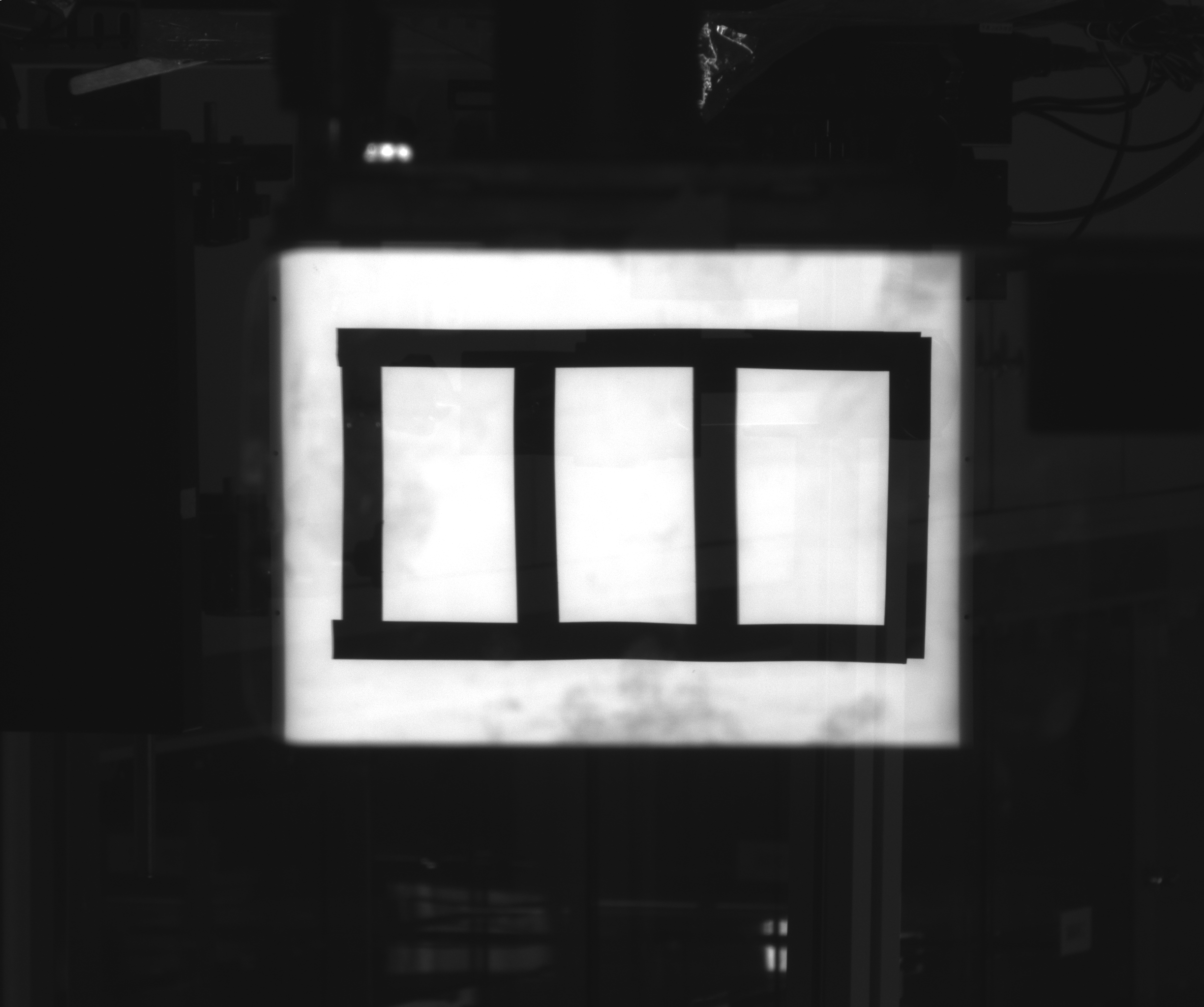
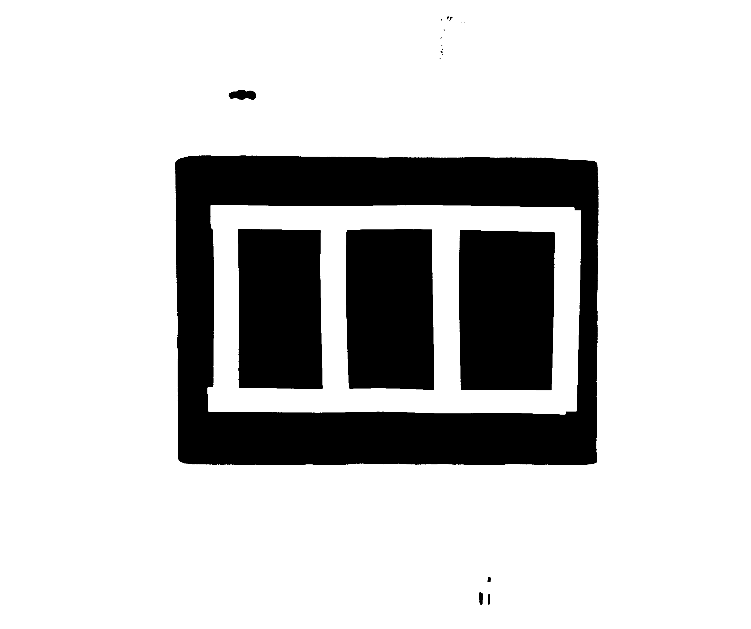
Figure 7.1 shows a typical scene: a panel under backlight illumination, where a dark tape grid stands out as a crisp silhouette against the bright light guide plate. A single automatic threshold extracts the tape grid cleanly as white foreground — no sophisticated algorithm required. This is precisely the promise of Chapter 4 — “proper lighting can reduce the problem to a single thresholding step” — being cashed in. But the other side of the same coin is this: thresholding’s dependence on gray values is so direct that its sensitivity to illumination changes is equally drastic. This chapter makes both sides of that coin concrete with a set of quantifiable experiments.

7.1 Global Thresholding and the Histogram

Global thresholding is thresholding in its plainest form: the entire image shares a single threshold \(T\). Taking the extraction of dark objects as an example,

\[ g[n,m] = \begin{cases} 255, & f[n,m] \le T,\\[2pt] 0, & f[n,m] > T. \end{cases} \]

The more general form is band thresholding: given an interval \([T_{\mathrm{low}}, T_{\mathrm{high}}]\), pixels whose gray values fall inside the band are foreground. A single threshold is just the special case \(T_{\mathrm{low}}=0\) (or \(T_{\mathrm{high}}=255\)).

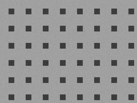
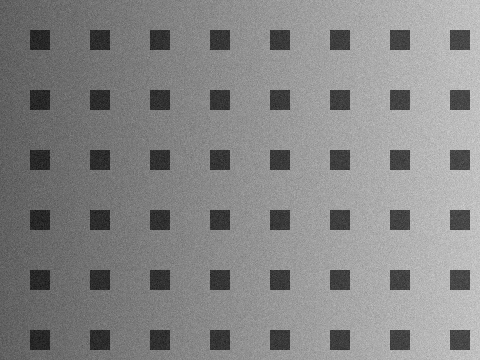
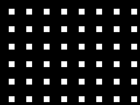
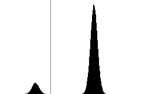
Where should \(T\) go? The answer hides in the gray-level histogram. If the object and the background are each uniform in gray value and clearly contrasted, the histogram shows two peaks — one for the foreground, one for the background — separated by a valley. This is the bimodal histogram. Place \(T\) at the bottom of the valley and the two populations are cut apart cleanly. The synthetic experimental scene of this chapter is designed exactly this way: on a \(480\times360\) image, a bright background of gray value 160 carries 48 dark squares of \(20\times20\) pixels (gray value 60, resembling a backlit dot calibration target), with additive Gaussian noise of standard deviation \(\sigma=6\) (fixed seed, reproducible); the ground-truth foreground totals 19200 pixels. Figure 7.2 (a) is the uniformly illuminated version; Figure 7.2 (b) is the same scene with a horizontal illumination gradient superimposed — a gain of \(\times 0.6\) at the left end and \(\times 1.2\) at the right, simulating uneven one-sided lighting.

\(T\) should sit in the middle of the valley, not at the foot of one of the peaks. With noise of \(\sigma=6\), each population spreads over roughly \(\pm 3\sigma=\pm18\) gray levels; place \(T\) too close to one peak and that population’s “long tail” will spill across it. Between 60 and 160, choosing \(T=110\) leaves 50 levels of margin to each peak — ample headroom.

A fixed threshold of \(T=110\) (band \([0,110]\)) performs flawlessly on the uniform scene: out of 172800 pixels, 0 are misclassified (Figure 7.3 (a)). But move to the gradient scene and the very same \(T\) goes bankrupt at once (Figure 7.3 (b)): at the left end the background gray value is pressed down by the gain to \(160\times0.6\approx96\), below 110, so roughly the leftmost 70 columns of background fall wholesale into the threshold band — 23728 pixels misclassified (13.73%), every one of them a false positive in which background is mistaken for foreground.

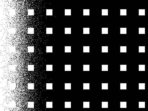
This controlled comparison spells out the precondition for fixed thresholding: stable illumination and controlled contrast. These two conditions are not granted by the algorithm — they are granted by the lighting design of Chapter 4: backlit silhouettes, narrow-band filters against ambient light, flat-field calibration — all of it exists to create the conditions under which “one \(T\) serves throughout”. When the conditions hold, a fixed threshold is the fastest and most predictable solution; when they do not, even the most painstakingly hand-tuned \(T\) is merely a down payment on the next illumination fluctuation.

7.2 Otsu’s Automatic Threshold

Choosing \(T\) by hand requires an engineer staring at the histogram and tuning. Otsu’s method automates that step: it sweeps every candidate threshold and picks the one that “separates the two populations the farthest”. Let \(p_i\) be the normalized histogram at gray level \(i\). A threshold \(T\) splits the pixels into two classes, whose proportions and means are

\[ \omega_0 = \sum_{i=0}^{T} p_i, \quad \omega_1 = \sum_{i=T+1}^{255} p_i, \quad \mu_0 = \frac{1}{\omega_0}\sum_{i=0}^{T} i\, p_i, \quad \mu_1 = \frac{1}{\omega_1}\sum_{i=T+1}^{255} i\, p_i. \]

Otsu’s criterion is to maximize the between-class variance:

\[ \sigma_B^2(T) = \omega_0\,\omega_1\,(\mu_0-\mu_1)^2, \qquad T^\ast = \arg\max_T \sigma_B^2(T). \]

Intuitively, \((\mu_0-\mu_1)^2\) rewards “the two class centers being far apart”, while \(\omega_0\omega_1\) penalizes lopsided splits where one class is large and the other tiny. By the variance decomposition of Chapter 2, the total variance \(\sigma^2 = \sigma_W^2 + \sigma_B^2\) (within-class plus between-class variance) is a constant independent of \(T\), so maximizing the between-class variance is equivalent to minimizing the within-class variance — making each class as internally compact as possible.

On the uniform scene, Otsu automatically selects \(T=86\), again with 0 misclassifications. Figure 7.4 shows where it lands: at the bottom of the valley between the two peaks — just as good as the hand-tuned result, but requiring no human intervention at all. When the illumination brightens or dims as a whole (for example, as a light source ages), both peaks shift together, and the \(T\) Otsu selects follows them automatically — this is its genuine advantage over a fixed threshold.

Figure 7.4: Gray-level histogram of the uniform scene. The small peak on the left is the foreground squares (centered near 60, 19200 pixels); the large peak on the right is the background (centered near 160). The vertical line marks Otsu’s automatically selected threshold \(T=86\), landing exactly in the valley between the two peaks.

But look at the result on the gradient scene (Figure 7.5): Otsu selects \(T=129\), misclassifying 52475 pixels (30.37%) — more than twice as bad as the fixed threshold’s 13.73%. The reason is not hard to see: the horizontal gradient smears the background gray value from a single 160 into a broad ramp spanning \(96\) to \(192\); the right-hand peak of the histogram is flattened into one continuous plateau, and the “two peaks with a valley” structure no longer exists. Otsu still faithfully maximizes the between-class variance, but on the distorted histogram, \(T^\ast=129\) falls inside the widened background mode — roughly the left third of the background has gray values below 129, and the whole stretch turns into false alarms.

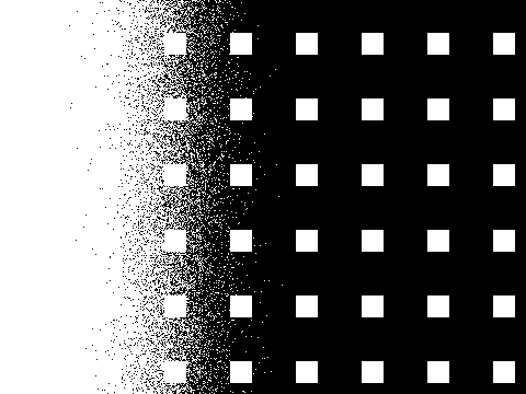
Figure 7.5: Otsu’s failure on the gradient scene: it automatically selects \(T=129\), a large swath of background on the left side of the image is mistaken for foreground, and 52475 pixels are misclassified (30.37%) — worse than the fixed threshold.

“Automatic” does not mean “adaptive”. What Otsu automates is the act of choosing \(T\), not adaptation to spatial variation — it still outputs a single global \(T\). The histogram is a statistic that erases spatial information entirely: what an illumination gradient destroys is precisely the premise that “pixels of the same class share the same gray value”, and no histogram algorithm, however clever, can repair that.

This is the most important teaching point of the chapter: Otsu’s implicit assumption is that the histogram is approximately bimodal. When the assumption holds, it is a tuning-free workhorse; when the assumption collapses, not only does it fail to save the day — its very appearance of being “automatic” makes it more deceptive. Engineers often realize only after a batch of misjudgments on the line that the automatically selected threshold had been sitting in the wrong place from day one.

7.3 Adaptive Thresholding

The essence of an illumination gradient is that the threshold ought to vary with position. Adaptive thresholding answers this head-on — instead of a global statistic, it opens a local \(K\times K\) window around every pixel and sets the threshold on the spot from the statistics inside the window. The most common form is “local mean minus an offset”:

\[ T[n,m] = \mu_K[n,m] - \beta, \]

where \(\mu_K\) is the local mean and \(\beta\) is a fixed offset. A pixel is judged (dark) foreground if it is darker than the average level of its own neighborhood by more than \(\beta\). Within the scale of the window, the illumination gradient is approximately constant: it raises the pixel value and the local mean by the same amount, so the subtraction cancels it automatically — exactly the “spatial adaptivity” that no global method can offer. The offset \(\beta\), in turn, suppresses noise in flat regions: without \(\beta\), about half the pixels on a uniform background naturally fall below the local mean, and a snowstorm of speckles erupts.

On the gradient scene, the result of local adaptive thresholding (\(K=81\), \(\beta=20\)) is shown in Figure 7.6: only 41 pixels misclassified (0.02%) — three orders of magnitude below the fixed threshold’s 23728 and Otsu’s 52475, with the squares at the darkest left end and the brightest right end extracted on equal terms.

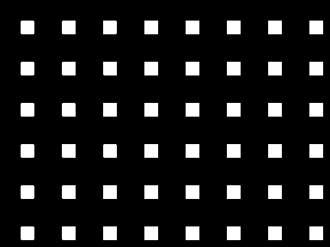
Figure 7.6: Local adaptive thresholding (\(K=81\), \(\beta=20\)) on the gradient scene: only 41 pixels misclassified (0.02%); the illumination gradient is cancelled automatically by the local statistics.

The window must be clearly larger than the object — a hard rule we established empirically: in this experiment, shrinking the kernel from 81 to 41 makes the interiors of the squares start to get “hollowed out”. When most of the window lies inside a \(20\) px square, the local mean itself approaches the square’s gray value, the center pixel is no longer darker than \(\mu_K-\beta\), and the square’s interior is judged background, leaving only a ring of outline. With 20 px objects, only a kernel of 81 is stable (the SDK’s local mean is center-weighted, so the effective window is smaller than the nominal size).

The price is two new parameters. The lower bound of \(\beta\) is set by the noise (it should exceed roughly \(3\sigma\); here \(\sigma=6\), so \(\beta=20\)), and its upper bound by the object contrast. The rule for \(K\) is in the margin note: the window must be larger than the object size, or the object’s interior gets hollowed out; at the same time the window must be smaller than the scale of the illumination variation, or the method degenerates back into global thresholding. Leave margin on both ends.

Finally, let us set this chapter side by side with the route taken in Chapter 4. Faced with uneven illumination, we now have two equivalent remedies: route one — first apply shading correction to flatten the background, then use a global threshold (the approach of Chapter 4); route two — skip the correction and apply local adaptive thresholding directly (the approach of this chapter). Their mathematical core is in fact the same — both “subtract a local estimate of the background”; the only difference is whether that step happens in the gray-value domain or in the decision domain. The engineering trade-off: if the corrected gray image will go on to serve other algorithms such as measurement or OCR, choose route one — one correction benefits the whole pipeline; if all you need is this one binary image, route two saves a processing stage and a round trip of an intermediate image through memory.

The four experiments are summarized below (172800 pixels total, ground-truth foreground 19200):

Method	Scene	Threshold	Misclassified (pixels)	Error rate
Fixed \(T=110\)	Uniform	110 (manual)	0	0%
Fixed \(T=110\)	Gradient	110 (manual)	23728	13.73%
Otsu	Uniform	86 (automatic)	0	0%
Otsu	Gradient	129 (automatic)	52475	30.37%
Adaptive \(K=81\)	Gradient	per-pixel	41	0.02%

7.4 Binarizing Color Images

The thresholding idea extends directly to color images: replace the single-channel band \([T_{\mathrm{low}}, T_{\mathrm{high}}]\) with one band per channel, and take the intersection of the three bands as the foreground — in RGB space this amounts to enclosing the target color in an axis-aligned box. The limitation of RGB is that all three channels are entangled with brightness; once the illumination changes, the box no longer contains the target. In practice the more robust approach is to convert to HSV space first: select the color with the hue channel, exclude gray and white regions with the saturation channel, and leave the brightness channel loose or unconstrained — color identity is thereby decoupled from illumination intensity, far more robust to lighting fluctuations than an RGB box. SciVision’s color binarization interface (SDK manual section 5.3) works in exactly this per-channel band-threshold fashion. The companion project of this chapter focuses on grayscale experiments and does not include a quantitative comparison for color binarization; only the principle is given here.

7.5 SciVision Implementation

The thresholding algorithms of this chapter are provided by the SCIMV::SciSvThreshold class. The fixed (manual) threshold call matches the companion project:

SCIMV::SciSvThreshold th;
SciImage dst;
SciROI roi;
SciPoint tl(0, 0), br(W, H);   // GenRect1 treats the bottom-right corner as exclusive: pass (W,H) for the full image
roi.GenRect1(tl, br);

// Band threshold [0,110]: pixels whose gray values fall inside the band become white (255) in the output
long rc = th.ManualThreshold(img, roi, 0, 110, SCI_THRESHOLD_TYPE_WHITE, 0, &dst);

In ManualThreshold(src, roi, lower, upper, lightOrDark, checked, dst), lower/upper are the bounds of the threshold band. The parameter name lightOrDark strongly suggests that it selects “extract bright objects or dark objects” — our tests show it does not: it controls the output coloring, not the object selection. Passing 0 (SCI_THRESHOLD_TYPE_WHITE) makes in-band pixels white (255) in the output. When extracting dark objects with the band \([0,110]\), you must pass 0 so that the objects come out as 255, consistent with the output convention of AutoThreshold (foreground is white); pass the wrong value and the binary image is inverted, and the connected-component statistics of Chapter 23 downstream will count the background as the object.

Automatic thresholding (Otsu and local adaptive) shares a single interface:

int t = -1;
// autoThresholdType=1: Otsu; the automatically selected threshold is returned via t (kernelSize/belta have no effect)
rc = th.AutoThreshold(img, roi, SCI_THRESHOLD_TYPE_BLACK, 1, 3, 5, 0, &t, &dst);

// autoThresholdType=6: local adaptive; kernelSize=81 is the window side length, belta=20 is the offset
rc = th.AutoThreshold(img, roi, SCI_THRESHOLD_TYPE_BLACK, 6, 81, 20, 0, &t, &dst);

Parameter	Meaning	Value used here, with notes
`lightOrDark`	Object polarity	`SCI_THRESHOLD_TYPE_BLACK` (extract dark objects)
`autoThresholdType`	Algorithm selection	1 = Otsu; 6 = local adaptive
`kernelSize`	Local window side length \(K\)	81 (must be clearly larger than the 20 px objects; 41 hollows out the squares)
`belta`	Local offset \(\beta\)	20 (should exceed the noise spread of roughly \(3\sigma\))
`value`	Output: the automatically selected threshold	Under Otsu, returns the selected \(T\) (86 on the uniform scene, 129 on the gradient scene)

Two engineering details deserve a dedicated record. The first is the lightOrDark semantics described above. The second is that SciROI::GenRect1 treats the bottom-right corner as an exclusive endpoint: a full-image ROI must be given \((W,H)\). If, following the intuition of “the coordinates of the last pixel”, you pass \((W-1,H-1)\), the last row and last column — \(W+H-1=839\) pixels in total — are excluded from processing and keep their original gray values: in the binary image this is an inconspicuous “leaky border”, yet more than enough to derail any pixel-by-pixel verification. The complete project that generates all experimental images of this chapter lives in code/thresholding/.

Industry Case: Threshold Drift in Backlit Measurement

A backlit dimensional-measurement station originally used a fixed threshold to extract the workpiece silhouette. After several months of operation, the measured dimensions began to drift slowly and systematically — the investigation traced it to aging of the backlight’s LEDs: brightness declined month by month, the contour cut by the fixed threshold expanded outward accordingly, and the dimensions were “measured larger” bit by bit. Switching to Otsu made the problem disappear: when the light intensity decays as a whole, both histogram peaks shift together, the automatic threshold follows, and the measurement stabilized. Then one day the line suddenly produced a batch of misjudgments: local contamination on the light guide plate dragged a long tail out of the background peak, the bimodal structure of the histogram was distorted, the threshold Otsu selected plunged into the background mode, and the contours of the entire batch were wrong — a live replay of this chapter’s gradient experiment. The final solution was Otsu plus a bimodality check: before every segmentation, verify the distance between the two histogram peaks and the depth of the valley, and raise an alarm and halt judgment whenever the metrics go out of bounds. “Automatic” must be paired with “self-checking” before it can run unattended on a production line.

7.6 Summary

Thresholding is the first step from pixels to objects: one gray-level threshold (or band) cuts the image into a binary foreground/background map. Its ceiling is set by the lighting — with stable illumination and controlled contrast, a fixed threshold is the fastest and most predictable (0 misclassified on the uniform scene); the moment the illumination develops a gradient, the same threshold fails outright (13.73%).
Otsu selects the threshold automatically by maximizing the between-class variance \(\sigma_B^2(T)=\omega_0\omega_1(\mu_0-\mu_1)^2\), and can follow global brightening or dimming of the illumination; but its implicit assumption is an approximately bimodal histogram. When that assumption collapses it can be worse than hand tuning (30.37% versus 13.73% on the gradient scene) — “automatic” does not mean “adaptive”.
Adaptive thresholding \(T[n,m]=\mu_K[n,m]-\beta\) cancels illumination gradients with local statistics (misclassification drops to 0.02%). The window \(K\) must be clearly larger than the object size, or the object’s interior gets hollowed out (kernel 41 fails; 81 is stable); \(\beta\) must exceed the noise spread.
There are two equivalent remedies for uneven illumination: shading correction followed by a global threshold (Chapter 4), or local adaptive thresholding directly (this chapter). Choose the former when the intermediate gray image has other uses; choose the latter when all you need is the binary image.
The binary image is a midpoint, not an endpoint: the remaining isolated specks and ragged edges are handed to the morphological cleanup of Chapter 8, and the aggregation of foreground pixels into objects and their measurement is the subject of Chapter 23.

The Otsu method used in this chapter comes from its 1979 original paper (Otsu 1979); for a systematic comparison and quantitative evaluation of the many thresholding methods, see the survey by Sezgin and Sankur (Sezgin and Sankur 2004); and for the place of thresholding within the overall digital-image-processing framework, see the textbook by Gonzalez and Woods (Gonzalez and Woods 2018). For a systematic treatment of thresholding and its connection to region-extraction algorithms, see the book by Steger et al. (Steger, Ulrich, and Wiedemann 2018).