15 The Hough Transform
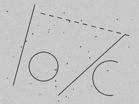
The search-line approach of Chapter 14 carries a self-evident premise: you roughly know where the target is. Frame an ROI first, then lay down the search lines — the whole pipeline rests on the prior of “one ROI, one primitive”. But what if that premise fails? The image contains multiple lines and multiple circles, with no advance knowledge of where each one sits; the targets may also be broken (dashed lines, gaps carved out by reflections) or partially occluded. Now there is nowhere to lay search lines, and point-by-point tracking snaps at the first gap. The Hough transform asks the question differently: instead of asking “where is this line”, it lets every edge point vote for all the lines that could pass through it (voting), and the parameter combination with the most votes naturally wins. This chapter runs the voting machinery end to end on a 480×360 synthetic scene (Figure 15.1): the scene contains 3 lines — one of them a dashed line with a gap ratio of about 47% — and 2 circles — one of them 40% occluded — plus 40 stray blobs and Gaussian noise with σ=8. Breaks, occlusion, clutter, and noise, all four kinds of interference present at once — exactly what it takes to force out the full value of the Hough transform.
15.1 Parameter Space and Voting
To vote for lines, the lines first need a suitable set of parameters. The Hough transform adopts the normal form parameterization (Duda and Hart 1972):
\[ \rho = x\cos\theta + y\sin\theta, \]
where \(\theta\in[0^\circ,180^\circ)\) is the angle between the line’s normal direction and the \(x\) axis, and \(\rho\) is the signed distance from the origin to the line. A pair \((\rho,\theta)\) uniquely determines a line, and both parameters are bounded: \(|\rho|\) never exceeds the image diagonal, and \(\theta\) needs only half a turn.
Why not the more familiar slope-intercept form \(y=kx+b\)? A vertical line has slope \(k\to\infty\), so the parameter space is unbounded in the \(k\) direction and cannot be discretized into a finite grid; moreover, a uniform partition of \(k\) corresponds to wildly non-uniform line directions (\(k\) from 0 to 1 sweeps 45°, while from 10 to 11 it sweeps only about 0.5°). The normal form keeps both parameters bounded and is uniform in direction — a parameterization tailor-made for voting.
The normal form brings a beautiful duality: substitute an image-space point \((x_0,y_0)\) into the equation above and let \(\theta\) range over \([0^\circ,180^\circ)\), and the resulting \(\rho(\theta)=x_0\cos\theta+y_0\sin\theta\) is a sinusoidal curve in parameter space — it enumerates all the lines passing through that point. Conversely, if a set of points is collinear on \((\rho^*,\theta^*)\), their sinusoidal curves must all pass through the very same point \((\rho^*,\theta^*)\) of parameter space. Detecting lines thus becomes finding the common intersections of a family of sinusoids.
The engineering realization is the accumulator: discretize the \((\theta,\rho)\) plane into a grid (e.g. 1°×1 px), initialized to zero; for each edge point, sweep over \(\theta\), compute the corresponding \(\rho\), and add one vote to the cell it lands in; once all points have voted, the peaks in the accumulator are the lines in the image — the vote count is the number of edge points lying on that line. A global geometric detection problem has been reduced to an array peak search.
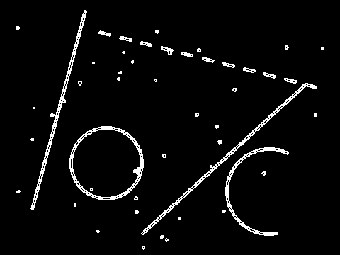
Where do the edge points come from? Any edge detector will do (the systematic treatment is Chapter 13) — this chapter thresholds the Sobel gradient magnitude of Figure 15.1 (threshold 200, about 7σ of the σ=8 noise level, anchoring the gate above the noise in the spirit of Chapter 7, with almost no false alarms), yielding 6677 edge points (Figure 15.2). Note that the gaps in the dashed line and the missing arc of the circle are preserved verbatim in the edge map — the voting is about to face them head-on.
15.2 Reading the Accumulator
Before calling the SDK, we build a 180×1201 accumulator by hand (1°/cell along \(\theta\), 1 px/cell along \(\rho\), \(|\rho|\le 600\)) and let the 6677 points vote one by one. The result is Figure 15.3: \(\theta\) on the horizontal axis, \(\rho\) on the vertical, gray levels stretched by a square root. Two layers of structure are visible: the family of sinusoidal curves filling the lower half — every faint bright curve is the voting trajectory of one (cluster of) edge points — and, within the family, three distinctly brighter intersections — the peaks of the three lines. The votes of the 40 stray blobs scatter along their own sinusoids, share no common intersection, and pile up into a peak nowhere.
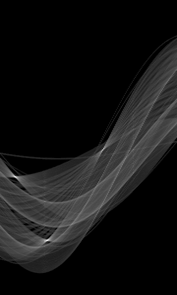
Do the peaks land where they should? From the ground-truth endpoints of the three segments we can predict each line’s \((\rho,\theta)\); we then extract the three largest peaks from the accumulator (global maximum + neighborhood suppression, refined to sub-cell accuracy with a 5×5 weighted centroid) and set them against the detections of the SDK’s FindHoughLines:
| Line | Predicted \((\rho,\theta)\) | Accumulator peak \((\rho,\theta,\text{votes})\) | SDK detection \((\rho,\theta)\) |
|---|---|---|---|
| L1 (solid) | (119.79, 15.00°) | (120.77, 15.30°, 291 votes) | (121.04, 15.01°) |
| L2 (dashed, 47% gaps) | (9.15, 104.25°) | (9.11, 104.25°, 190 votes) | (9.22, 104.01°) |
| L3 (solid) | (378.55, 47.60°) | (377.31, 48.05°, 260 votes) | (379.19, 48.02°) |
All three lines pass verification: the \(\theta\) deviation stays within half a degree, the \(\rho\) deviation within 1.3 px. That 1.3 px is no mystical error floor; it has a definite origin: the strokes in the scene are about 2.8 px wide, and Sobel detects a row of edge points on each side of the stroke; the two rows are each collinear, about 2.8 px apart, and the post-voting peak is a compromise between the two rows of votes, so its position drifts between the sides — the accumulator’s peak is forever faithful to the geometry of the edge points, and the geometry of the edge points is dictated by the stroke width.
The row most worth staring at is L2: the dashed line is missing 47% of its stroke, and its vote count drops from the solid lines’ roughly 290 to 190, yet the position of the peak does not budge and remains clearly identifiable. This is the soul of the Hough transform — break immunity. Voting only asks “does this point lie on this line”, never “is it connected to its neighbors”: gaps merely shave votes off in proportion; they do not move the peak, let alone make it vanish. By contrast, any method that relies on local continuity (edge tracking, contour linking) snaps at the first 14 px gap. Global evidence accumulation and local continuity tracking are two worldviews; when the target is inherently broken, only the former is left standing.
15.3 Multiple Instances and Robustness
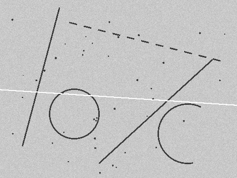
What happens if, instead of voting, we hand “find the lines” to our most familiar tool, least squares? Run a negative experiment: fit one total-least-squares line to all 6677 edge points at once, and the result is \(\rho=180.04\), \(\theta=93.76°\), with an all-point RMS distance of 82.6 px — the white line slashing across the image in Figure 15.4, matching none of L1, L2, or L3. This is not an implementation slip; the question itself was wrong: least squares assumes all points obey one and the same model, while the points here belong to three lines, two circles, and 40 stray blobs; “the optimal single line over all points” is a compromise for an object that does not exist — it can only land near the centroid of all the structures, oriented along the principal axis of greatest scatter — an “average line” that is nobody.
The Hough transform is born without this dilemma: each instance gathers its own peak in the accumulator, none interfering with the others — L1’s 291 votes, L2’s 190, and L3’s 260 each sit in their own place; points that belong to no line — the circle arcs and the clutter — scatter their votes everywhere and never form a peak. Multi-instance separation and robustness to clutter are two faces of the same mechanism: concentrated votes win, scattered votes lose. Figure 15.5 shows the detections of the SDK’s FindHoughLines: all three lines are hit (white lines), the dashed one included.
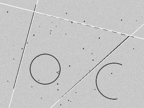
FindHoughLines (white lines; the infinite lines are clipped to the image borders). The dashed line L2 is detected as usual despite its 47% gaps; the circles and the clutter produce no false alarms.
How do Hough and the robust fitting of Chapter 14 (Huber, RANSAC) divide the work? Robust fitting handles “one instance + a few outliers”, still under the premise that an ROI has roughly framed the target, with subpixel accuracy as the reward; RANSAC can handle multiple instances by “find one, remove its inliers, find the next”, but turns inefficient once instances multiply. Hough handles “an unknown number of instances + plenty of irrelevant structure”, needs no positional prior whatsoever, at the cost of accuracy capped by the accumulator quantization. Rule of thumb: have an ROI and need accuracy — search lines + robust fitting; no prior and need to find them all — Hough.
15.4 Hough Circles
A circle has three parameters \((c_x,c_y,r)\), so the accumulator rises from two dimensions to three: an edge point’s voting trajectory is no longer a sinusoid but a cone surface in parameter space (the farther a candidate center lies from the point, the larger the required radius). A direct implementation costs an order of magnitude more than the line case in both memory and vote counting, so practical algorithms almost universally accelerate with the gradient direction: an edge point’s gradient points toward (or away from) the circle center, so votes need only be cast for candidate centers along the gradient ray — the 3D problem collapses into two steps, “2D center accumulation + 1D radius histogram”, which is exactly the 2-1 Hough strategy adopted by mainstream implementations (including OpenCV and most industrial libraries).
A feel for the magnitudes: for a 480×360 image and a radius search range of 40 px, a naive 3D accumulator has 480×360×40 ≈ 6.9 million cells, and every edge point must draw a full circle of votes in every radius layer; with gradient-direction acceleration, each point casts only a few dozen votes along a single ray. Without this step, Hough circles cannot run within a production-line cycle.
The experiment continues on the same scene (Figure 15.6): FindHoughCircles detects exactly two circles. The complete circle C1 has ground truth \((150,230,50)\) and is detected at \((151.0,231.0,50.2)\) — a center error of 1.41 px and a radius error of 0.20 px; C2, missing 40% of its arc, has ground truth \((380,270,60)\) and is detected at \((377.0,267.0,57.8)\) — a center error of 4.24 px and a radius error of 2.20 px. The two sets of numbers add up to one sentence: under occlusion, accuracy degrades, but detection does not fail. The cause of the degradation is the same as the line’s ρ shift, only stronger: the circle’s three parameters are mutually coupled, the missing arc tilts the vote mass toward the surviving arc, and the peak gets pulled slightly off; but the remaining 60% of the arc still contributes enough votes to gather into a peak — break immunity replayed on circles.
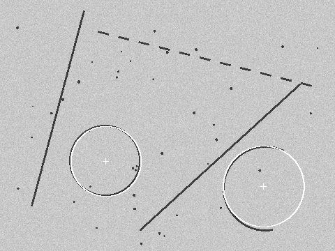
FindHoughCircles (white circles and crosses mark the detected circles and centers). The complete circle C1 has errors of 1.41/0.20 px; C2, missing 40% of its arc, has errors of 4.24/2.20 px — under occlusion accuracy degrades but detection does not fail.
The essential ceiling on accuracy must also be seen clearly: measurements show this SDK’s circle centers are quantized to a 2 px grid and its radii step by about 0.2 px — the direct imprint of the accumulator cell size; no number of votes can buy resolution below the cell. Hence the standard industrial recipe is two-stage: Hough for coarse localization, search lines for precise measurement — first use Hough to find every circle across the whole image (no prior needed, occlusion-tolerant), then take the detected center and radius as the prior to construct an annular ROI and hand it to the radial search lines + robust fitting of Chapter 14 for subpixel-precise measurement. Hough answers “where”, search lines answer “how precisely” — the methods of the two chapters are not rivals but upstream and downstream of one pipeline.
15.5 SciVision Implementation
Hough lines are provided by SCIMV::SciSvHoughLines, which performs Canny edge extraction internally and consumes the gray image directly:
SCIMV::SciSvHoughLines houghL;
SciPointArray term;
SciVarArray lineAng, lineLen;
long rc = houghL.FindHoughLines(src, fullROI, /*cannyLow*/ 60, /*cannyHigh*/ 120,
    /*accumThreshold*/ 65, /*minAngle*/ -90, /*maxAngle*/ 90,
    /*AngleGap*/ 5, /*DistGap*/ 10, /*maxNum*/ 6, /*AngleCheck within range*/ false,
    &term, &lineAng, &lineLen);
cannyLow/cannyHigh are the dual thresholds of the internal Canny; accumThreshold=65 is the vote-count gate — peaks with fewer than 65 votes are not reported; minAngle/maxAngle bound the accepted range of line angles; AngleGap=5 and DistGap=10 define the neighborhood for peak deduplication (peaks differing by <5° in angle and <10 px in distance are merged into one line); maxNum=6 caps the number of lines returned. In this example up to 6 lines were allowed and exactly the 3 ground-truth lines were detected — no false alarms under these parameters.
In actual testing this API exhibits three behaviors that contradict intuition (or the documentation) and must be recorded honestly. First, the header file does not state what the values of AngleCheck mean: measurement shows that false means “find lines within the angle range” and true means find those outside it — passing true together with the full range [-90,90] directly yields the “no suitable line found” error code 122408001. Second, the default Canny thresholds 20/40 fail on this scene: under σ=8 noise there are too many false edge points, the votes of the real lines drown in noise votes, and phantom diagonal lines spanning the whole image surface in the accumulator; results only stabilize once the thresholds are raised to 60/120 — the Canny gate must be anchored above the noise level, the same reasoning as the 7σ threshold of the hand-built edge map in Section 15.1. Third, the semantics of the return values: the “endpoints” in term are not segment endpoints but the intersections of the infinite line with the image borders (which is why every white line in Figure 15.5 runs clear across the image), and lineLenth is the clipped length; the angle returned in lineAng is \(90^\circ-\theta\) (the line’s direction angle, not the normal angle) — do not get the conversion backwards.
Hough circles are provided by SCIMV::SciSvHoughCircles:
SCIMV::SciSvHoughCircles houghC;
SciPointArray centers;
SciVarArray radii;
rc = houghC.FindHoughCircles(src, fullROI, /*minDist*/ 100, /*edgeThreshold*/ 160,
/*accumThreshold*/ 65, /*minRadius*/ 35, /*maxRadius*/ 75, /*maxNum*/ 4,
¢ers, &radii);minDist=100 is the minimum spacing between two circle centers (deduplication); edgeThreshold is the strength gate of the internal edge extraction; accumThreshold=65 is the vote-count gate of the center accumulator; minRadius/maxRadius delimit the radius search band of 35–75 px. There is a pitfall here as well: the default edgeThreshold=80 is too low — noise edges gather into phantom circles whose radius hugs maxRadius (a large-radius circle has a long circumference, more noise points happen to pass by, a built-in vote advantage); after raising it to 160 and pairing it with accumThreshold=65, only the two ground-truth circles are detected even with maxNum=4 left open. A final reminder about the output quantization granularity: centers land on a 2 px grid and radii step by about 0.2 px — the moment you receive the result you should know it is a “coarse localization”, and leave the precise measurement to the downstream. The complete project that generates all of this chapter’s images and numbers lives in code/hough_transform/.
Industry Case: Counting Pins on a Tray
An IC tray inspection station must count the pins of each chip in its pocket: under ring light the metal pins reflect and image as a set of intermittent short bright lines — each pin breaks into two or three segments, and the count varies with the chip model. Template matching does not apply (the pin count is variable and the appearance changes with the reflections), and search lines have nowhere to lay their ROIs. Hough lines fit exactly: the pin direction is known (perpendicular to the chip body), so narrowing minAngle/maxAngle to an angular band of ±10° around that direction throws out reflections in irrelevant directions from the start; the several broken bright segments pool their votes into the same peak in the accumulator — break immunity automatically merges “several segments” back into “one pin”; finally the vote-count gate filters out sporadic reflections, and the number of detected peaks is the pin count. The center of gravity in tuning is exactly the same as in this chapter’s experiments: first measure the noise level of the production-line images and anchor the internal Canny thresholds above it — the moment phantom lines appear, the count can no longer be trusted.
15.6 Summary
- The Hough transform turns geometric detection into voting: under the normal form \(\rho=x\cos\theta+y\sin\theta\), an image point is dual to a sinusoid in parameter space, and the sinusoids of collinear points intersect at a single point; a discrete accumulator counts the votes, and the peaks are the lines.
- Break immunity is the Hough transform’s soul: voting only checks “on the line or not”, never “connected or not” — gaps cut votes but do not move peaks. The dashed line with 47% gaps still peaked with 190 votes, and the 40%-occluded circle was detected as usual.
- Multi-instance separation and clutter robustness are the same mechanism: each instance gathers its own peak, scattered votes gather into none; in the negative experiment, a single-line least-squares fit to the 6677 points produced an “average line” with RMS 82.6 px — on multi-instance data the optimum over everything is a meaningless compromise.
- Hough accuracy is capped by the accumulator quantization (here circle centers on a 2 px grid and radii in 0.2 px steps; the line’s ρ deviation is further swayed by the votes from the two sides of the stroke), so the engineering recipe is “Hough for coarse localization + search lines for precise measurement”, forming an upstream–downstream pair with Chapter 14.
- Anchor parameters to the noise and verify semantics empirically: internal Canny thresholds below the noise level breed phantom lines/circles; this chapter’s SDK has
AngleChecksemantics opposite to the documentation, returns border-clipped intersections as endpoints, and reports the angle as \(90^\circ-\theta\) — always validate critical semantics on synthetic images with known ground truth before going live.
The original reference for the Hough transform is the classic paper by Duda and Hart (Duda and Hart 1972); its generalization from lines to arbitrary shapes is Ballard’s generalized Hough transform (Ballard 1981), and Illingworth and Kittler’s survey systematically maps the variants and computational strategies (Illingworth and Kittler 1988). For its connection to geometric measurement pipelines, see further the book by Steger et al. (Steger, Ulrich, and Wiedemann 2018).