42 3D Inspection
The inspection part (Part VI, where Chapter 26 lives) hammered the paradigm of defect detection into a single sentence: a defect is a deviation from “normal” — first define the one and only normal, then quantify the endlessly varied deviation. The stage there was a 2D grayscale image, where both normal and deviation were written into pixel brightness. This chapter carries the same paradigm into three dimensions: the object under test is no longer a grayscale image but a range image (height map) — each pixel stores not brightness but the true height (mm) of the object’s surface at that point. Not a word of the paradigm changes, yet the dimensionality does: in 3D a defect acquires, for the first time, height, volume, and flatness — quantities that 2D grayscale simply cannot see. An ink blot 25 gray levels darker than its background can only be told apart in 2D through contrast; but a 0.99 mm step or a 7 mm boss is, in 3D, 0.99 mm and 7 mm — no more, no less. Dimension equals physical quantity, and this is the deepest dividend of 3D inspection over 2D, the thread that runs through this entire chapter.
This chapter runs all its experiments on a real Smart3 range image (Figure 42.1, file 001.srt from the Smart3 1.9.2.2 “3D multi-contour inspection” sample recipe): the part under test is a multi-level molded/machined component, with a top-view field of 32 mm×50 mm, a lateral resolution of 0.02 mm/px (1600×2500), and a height resolution ResolutionZ of only 0.01 µm/count (extremely fine quantization). It is “multi-contour” in the literal sense — the surface splits into an upper and a lower plateau (a step of about 1 mm), bearing several contour features of wildly different heights: a tall central boss (about 7 mm above the reference surface), a low boss on the lower plateau, a recessed racetrack groove at the top end together with the raised platform it encloses, and a few tiny pits on the tall boss’s top face. Figure 42.1 spreads the levels out at a glance with a jet height encoding: deep blue is the lower plateau, light blue the upper plateau, the central boss dyed deep red rises high, the cyan low boss sits at the bottom, and the racetrack contour at the top is clearly visible. Worth noting is that only 41.3% of the pixels are valid: the other 58.7% are marked invalid (raw count INT_MIN), corresponding to steep walls, deep bores, and laser no-return regions — this is the biggest difference between real 3D data and synthetic data, and every step below must first answer “does this pixel have data.”
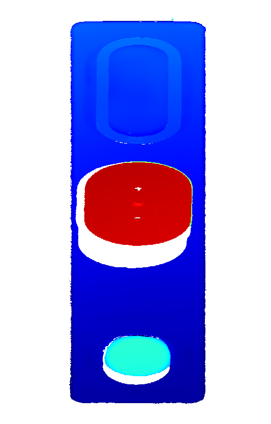
001.srt, 1600×2500, jet height encoding). The part splits into an upper and a lower plateau; the central deep-red feature is a boss about 7 mm above the reference surface, with tiny pits visible on its top face; the cyan feature at the bottom is the low boss; the racetrack contour at the top is a raised platform enclosed by a recessed groove. White is invalid pixels (steep walls/no-return, 58.7%). Lateral 0.02 mm/px, field 32×50 mm.
A range image is also called 2.5D data: it stores a single-valued height \(z(x,y)\) on a regular \(x,y\) grid, sitting between a 2D image (no height) and a full 3D point cloud (Chapter 37, where each point may have arbitrary \(x,y,z\) and can express overhangs and closed surfaces). The native output of laser triangulation (Chapter 33), structured light (Chapter 32), and similar devices is mostly exactly a range image — this chapter assumes it has already been produced and focuses on “once you have the range image, how do you judge contours and defects.” At steep walls and deep bores the laser gets no return, and the sensor can only mark the pixel invalid (here with INT_MIN); the valid-pixel fraction varies wildly with the workpiece relief.
42.1 Multi-Contour Segmentation: 3D Blob Analysis
Two-dimensional blob analysis (Chapter 23) is a three-step pipeline of “threshold segmentation + connected components + feature measurement”: binarize the image, then organize the heaps of white pixels into objects and measure them. The first tool of 3D inspection is almost its word-for-word counterpart, except the basis for segmentation switches from “grayscale over threshold” to “height deviation over threshold” — which is exactly the heart of “multi-contour inspection”: cut one range image into a set of contour regions of wildly different heights, then measure each one.
Concretely, first estimate a reference surface — the median of all valid heights is a robust baseline (measured \(h_\text{ref}=-1.694\) mm, landing right on the largest-area upper plateau; the median is immune to a handful of tall feature pixels). Then compute the per-pixel deviation \(\Delta h(x,y)=h(x,y)-h_\text{ref}\); pixels with \(\Delta h\) above \(+\tau\) are “raised candidates,” those below \(-\tau\) are “recessed candidates,” and connected-component analysis runs on them separately (raised and recessed apart, to keep an adjacent raised region and recessed region from merging into one blob at their boundary). The tolerance is set at \(\tau=0.35\) mm and the minimum area at 1500 px (0.6 mm²) to filter out debris.
What a 3D contour has beyond a 2D blob is precisely the new criteria that height brings. Besides the 2D suite of area, centroid, and bounding box, each contour also yields: a signed height deviation (the sign of the mean distinguishes a raised contour \(\Delta h>0\) from a recessed one \(\Delta h<0\), information a 2D binary image inherently throws away), an equivalent diameter, and a volume \(V=\sum_{(x,y)}\Delta h(x,y)\cdot A_\text{px}\) (where \(A_\text{px}=0.02\times0.02=4\times10^{-4}\) mm² is the pixel area, the unit is mm³, and it answers directly “how much material does this contour stick out or sink in”).
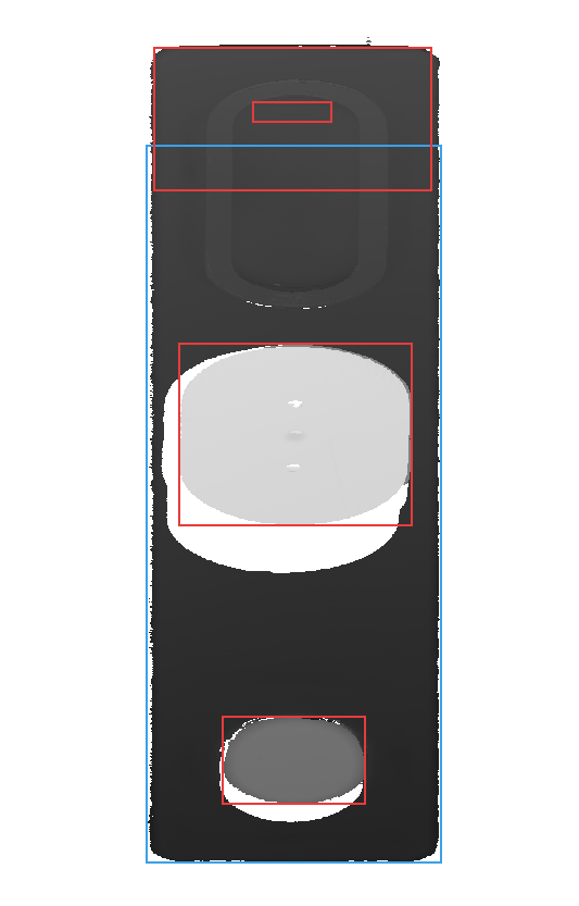
The measurement segments 5 contour features from this real range image (Table 42.1, Figure 42.2): the most prominent is the central boss — equivalent diameter 11.76 mm, 7.15 mm above the reference surface, volume 776 mm³, the geometric protagonist of the whole part; the low boss on the lower plateau has an equivalent diameter of 6.23 mm and a height of 2.22 mm (bounding box 7.8×4.8 mm, slightly racetrack-shaped); the raised platform enclosed by the racetrack groove at the top spans 54.7 mm² and is only 0.47 mm high; and the whole lower plateau, as a large recessed contour (247 mm², mean −0.89 mm), is faithfully separated out — it is the low side of that roughly 1 mm step.
| # | Type | Area mm² | Eq. dia mm | Center (x,y) mm | Mean Δh | Peak Δh | Volume mm³ |
|---|---|---|---|---|---|---|---|
| 1 | Raised | 108.6 | 11.76 | (16.3, 24.0) | +7.145 | +7.696 | +775.9 |
| 2 | Recessed | 247.0 | 17.74 | (16.6, 37.3) | −0.892 | −3.868 | −220.3 |
| 3 | Raised | 54.7 | 8.34 | (15.9, 5.1) | +0.465 | +0.917 | +25.5 |
| 4 | Raised | 30.5 | 6.23 | (16.2, 41.9) | +2.222 | +2.428 | +67.8 |
| 5 | Raised | 2.6 | 1.81 | (16.0, 6.2) | +0.367 | +0.406 | +1.0 |
Here the fundamental advantage of 3D inspection emerges: the criteria are closer to physical quantities. 2D blobs classify by pixel-geometry quantities such as area and circularity, which shift with resolution and viewpoint; a 3D contour’s height (mm), volume (mm³), and equivalent diameter (mm) are calibrated true dimensions (exactly the “3D metrology gives physical units directly” stressed in Chapter 41). A line such as “boss height must be 7±0.1 mm, step must be 1±0.05 mm” can be written into the process specification verbatim, with no translation into pixels — the unification of dimensionality lets the rulebook and the algorithm speak the same language.
In practice a volume criterion is often more robust than a height criterion: a sharp tall burr (large height, small volume) and a shallow broad swelling (small height, large volume) usually carry different risks, and looking at peak height alone conflates them. Using height and volume as a dual criterion — “NG if height exceeds A or volume exceeds V” — fits the real question of “will this contour cause a failure” better than any single criterion. Here the central boss’s 776 mm³ versus the low boss’s 67.8 mm³ reflects their disparity in bulk far more vividly than their diameters do.
42.2 Cross-Section Measurement
Blob analysis answers “where the contours are and how large their volume,” but a production line often needs a sharper question still: along a specified straight line, what exactly does the surface height profile look like? This is profile/cross-section measurement — extract the height sequence along a line segment on the range image to obtain a one-dimensional profile curve. It is the caliper of the three-dimensional world (Chapter 20): a caliper finds edges and measures distances along a search line on a grayscale image, while a cross-section reads heights and measures steps and peaks along a line on a range image. The two are isomorphic — both reduce 2D/3D data along a line down to 1D, then resolve it with classical one-dimensional signal tools.
The experiment extracts a cross-section along the vertical center line \(x=16.1\) mm, which passes through both the tall and the low boss (Figure 42.3). This line walks through every level in one stroke: the upper plateau, the top groove, the raised platform, the central boss top rising sheer (including the two downward notches of the pits on its top face), the step plunging to the lower plateau, then climbing onto the low boss. The measured profile has 2054 valid points, with a height range of [−6.562, 5.987] mm: the boss top peaks at 5.987 mm (at \(y=22.2\) mm), 7.66 mm above the upper plateau (−1.668 mm); the upper-to-lower plateau drop is the step height of 0.988 mm. All of this is clearly readable in Figure 42.3: two horizontal reference lines mark the two plateaus, the sheer raised platform in the middle is the boss top (red dot marks the peak), the two downward notches on the boss top are precisely the pits inspected next, and the half-height step on the right is the low boss.
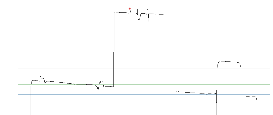
Worth a special note: of this chapter’s three SDK 3D inspection modules, the only one measured working is cross-section measurement. SciSv3DProfileMeasure::ExtractData returns rc=0, 2054 sample points, and a Z range of [−6.562, 5.987] mm along the same line — point-for-point identical to the hand-written row-by-row column read — because it is stateless, merely “read along a line + interpolate,” and is therefore robust and usable. The value of a cross-section is more than “reading the profile”: once 2.5D data is reduced along a line back to 1D, the full suite of one-dimensional subpixel tools of Chapter 14 becomes available — parabolic fitting at a peak yields a subpixel peak position, an edge model measures step width and slope, and a line fit to a baseline segment estimates tilt. The cross-section is the bridge connecting three-dimensional data with classical one-dimensional metrology tools.
Where to draw the cross-section line is an engineering decision, not an algorithm problem. A section through the deepest part of a defect gives the maximum deviation, a section along a workpiece edge checks steps and edge collapse, a section perpendicular to a scratch measures groove depth and width. In practice one often first takes a contour centroid from Section 42.1, then automatically lays a section line (or a fan of them) at the centroid for fine measurement — the contour “finds it,” the cross-section “measures it precisely,” a division of labor identical to the 2D pattern of “blob to locate, then caliper to measure precisely.” This chapter’s center line is information-dense precisely because it threads every level on a single stroke.
42.3 Local Defects and Surface Quality
The previous two sections answered “which contours there are, and how large each is,” but inspection has a finer layer still: for a face that is supposed to be flat, is it itself flat, and does it have local blemishes? This pulls the scale of inspection from “between contours” into “within a single contour.” This section uses the central boss’s top face as its stage — nominally a flat circular land, it is the purest exercise of the paradigm “define the one and only normal, then quantify the deviation”: first fit the top face itself into “normal,” then dig out the local dips that deviate from it.
The method has two steps. First, fit the top face into a reference plane. Take the boss with a height threshold (\(z>1.5\) mm) and connected components, then erode inward by 14 rings to strip off the slanted walls and edges (leaving only the clean interior top face, 96.85 mm²), and least-squares-fit it to a plane \(z=ax+by+c\). The fitted top face carries about a 1.4° clamping tilt (\(a,b=-0.0074,-0.0230\)); with the tilt removed, the top-face residual has a flatness RMS of only 15.4 µm — on a 7 mm-tall boss top quantized at 0.01 µm, this is a remarkably flat face. Second, flag the local dips that deviate from the reference plane as defects: pixels whose residual is below \(-0.25\) mm are “pit candidates,” counted by connected components. The measurement detects 2 pits: one of area 0.440 mm² and depth 644 µm, and one of area only 0.014 mm² and depth 818 µm. Figure 42.4 is a diverging-colormap heat map of the top-face residual (blue = dip, red = bump, white = flush with the reference plane): the whole top face is mostly white (proof that it really is flat), with only the blue-cored red-rimmed patch at the center being the 0.44 mm² pit, and the small dot boxed in black below it being the 0.014 mm² micro-pit; the white void near the top is a laser-no-return deep bore on the top face (invalid pixels, not counted as a pit).
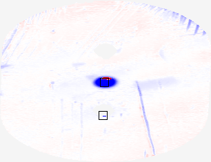
This section pushes the paradigm of defect detection to its logical end: “normal” need not be the nominal value on a drawing; it can be a reference plane fitted on the spot from the data. The top-face flatness RMS of 15.4 µm and the pit depths of 644/818 µm are two physical quantities of the same dimensionality, each directly thresholdable against a drawing tolerance — the former answers “is this face flat enough,” the latter “is there any damage.” One sentence closes this section, and closes the methodology of the entire inspection part: the definition of a defect determines what quantity, and against what baseline, you use to measure it.
The SDK has a module named “concentration/density detection” (SciSv3DConcentrationDetection), meant to detect statistical defects — blemishes whose mean is normal and only the local variance is anomalous (local polishing on a matte surface, orange peel in coatings, porosity in sintered parts), caught by local height variance rather than a height threshold. But on this machine it is silent with no output (see Section 42.5), so this chapter demonstrates the same paradigm by the geometric route (residual flatness + pits). Statistical and geometric defects share the same essence — “define normal first, then quantify the deviation” — only the former writes the “deviation” into variance and the latter into height; use the wrong ruler, and even the best algorithm merely computes a zero error precisely.
42.4 Detection Limit and Minimum Detectable Size
The two pits detected in Section 42.3 differ greatly in size: one is 0.440 mm², the other only 0.014 mm² (about 35 pixels, 3–4 pixels wide). The latter already hugs this system’s detection limit — it asks not “how deep” but “how small before it can no longer be detected.”
First, see the nature of the limit clearly. Both pits are 600–820 µm deep, far above the top face’s 15 µm flatness noise floor (SNR about 40), so “whether it is detected” is unrelated to depth; the real bottleneck is lateral size and the connected-component minimum-area floor. Sweeping the pit-detection minimum area \(A_\text{min}\) across tight, default, and loose settings (depth threshold fixed at 0.25 mm) gives:
| Setting | Min area | Pits detected | Stray specks (≥1 px) |
|---|---|---|---|
| Tight | 6 px | 2 | 0 |
| Default | 25 px | 2 | 0 |
| Loose | 200 px | 1 | 1 |
This table gives a conclusion strikingly different from synthetic data, and more honest too. In the 2D world of Chapter 26, the threshold dilemma was “tight = false alarms, loose = missed detections” — tighten the threshold and noise spikes cross the line in patches. But this high-quality real scan’s top face is so clean that even pushing the minimum area down to 6 px raises no noise specks at all (false alarms = 0). In other words, there is no false-alarm-versus-miss dilemma here, only a one-sided size floor: the loose setting (200 px) drops the 0.014 mm² micro-pit outright (only 1 detection remains), and what truly decides “the smallest detectable” is the 0.02 mm lateral resolution itself — a 3–4-pixel-wide pit already approaches the boundary where “a single dropped pixel versus a real pit” becomes hard to tell apart. Figure 42.5 puts the two settings side by side: the left (tight, 6 px) boxes both pits, the right (loose, 200 px) keeps only the central large pit, with a blank where the micro-pit sits.
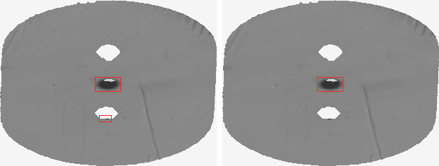
The tuning method still descends from the “squeeze from both ends” of Chapter 26: use the smallest known real defect to verify detection and get the upper bound (the size floor), and use good parts to press down false alarms and get the lower bound — only this clean scan’s false alarms are already zero, the lower bound is loose, and the whole bottleneck sits in the upper bound (lateral resolution). To push this size floor lower, what should change is not the area threshold but the acquisition scheme: a lens with higher lateral resolution and a denser scan-line pitch (the sensor selection of Chapter 30 exists precisely to pry this window open). And on this question 3D inspection still holds a card 2D does not: the depth criterion is in physical units (µm) — “pit depth must be < 100 µm” is an absolute process quantity reproducible across devices, not drifting with illumination or exposure, which makes 3D threshold tuning steadier and more portable than a 2D grayscale threshold.
The “detection limit” of real data often lies not in the algorithm but in the sampling: the 58.7% invalid pixels (steep walls/deep bores with no return) are the first wall you hit. That no-return deep bore on the top face is the proof — it is not a defect, yet it is a thorough data void that any top-face flatness assessment must exclude first. A 3D inspection engineer’s first homework is usually “where is there no data,” and only second “is the data that exists judged accurately.”
42.5 SciVision Implementation
This chapter records faithfully the measured state of three SciVision 3D inspection modules on this machine, against this real range image — itself the book’s last practice of its methodology: every promise of a commercial library must pass a golden experiment.
// Load the real range image (link Sci3DFileOperation.lib; rc=0 means success;
// it prints a harmless "Directory does not exist." to stderr)
SciRangeImage ri; SCIMV::Sci3DFileOperation fop;
long rc = fop.LoadRangeImage(SciVar("sample\\001.srt"), &ri, false);
double z = ri.GetValue(r, c) * ri.ResolutionZ(); // raw count × Z-resolution = physical height mm
// invalid pixels are marked INT_MIN(-2147483648) (steep walls/no-return); must be excluded explicitly
// ① Cross-section measurement (measured working! extracts height data along a line)
SciROI line; line.GenLine(SciPoint(805,120), SciPoint(805,2380));
SCIMV::SciSv3DProfileMeasure pm; SciFloatArray wz; /* ... */
rc = pm.ExtractData(ri, line, shield, 0, 0, &wxy, &ixy, &wz, NULL, &idxZ, &dist, NULL);
// rc=0, wz.Length()==2054, Z∈[-6.562,5.987]mm —— point-for-point identical to the hand-written profile
// ② 3D blob analysis (measured silent: rc=0 but blobs.Length()==0)
SCIMV::SciSv3DBlobAnalysis ba; SciRegionArray blobs; SciMatrix res;
rc = ba.BlobAnalysis3D(ri, roi, base, lo, hi, mn, mx, ft, rt,
false, false, &blobs, &res); // rc=0, blobs=0, res 0×0
// ③ Concentration/density detection (measured silent: rc=0 but dst is a 0×0 empty image)
SCIMV::Sci3DConcentrationDetection cd; SciImage dst; /* ... */
rc = cd.DetectConcentration(ri, roi, 0.05, 9,
SCI_CONCENTRATION_FILTER_MEAN, 4, 4, &diff, &dst, ®); // dst 0×0The measured conclusions are clear-cut: SciSv3DProfileMeasure::ExtractData is working — it returns 2054 sample points along the specified line segment, with a Z range of [−6.562, 5.987] mm, point-for-point identical to the hand-written profile, the only 3D inspection primitive among the three modules that can be used directly in production. Whereas SciSv3DBlobAnalysis::BlobAnalysis3D and Sci3DConcentrationDetection::DetectConcentration are both silent with no output — the return code is rc=0 (nominal success), but the former’s blobs has length 0 and the latter’s dst is a 0×0 empty image, with no actual output whatsoever. This matches the “silent no-output” signature of several 3D modules in Part IX, so this chapter’s main algorithms are all hand-written fallbacks: height-deviation connected-component analysis for multi-contour segmentation (Section 42.1), and least-squares top plane + residual for flatness and pit detection (Section 42.3). To isolate the silent/crash risk, all three SDK modules are invoked through a subprocess probe — the main flow first system()s a subprocess to run the probe and records its return and output, then proceeds with the hand-written algorithm, so that no SDK anomaly can drag down the main flow. This engineering posture is itself a conclusion: the SDK maturity of current 3D inspection is markedly below that of 2D, and most inspection operators still need to be self-developed — no surprise, since 3D inspection is the youngest piece of machine vision, and a standardized operator library is still taking shape.
Why is the cross-section working while the blob and concentration are silent? A reasonable guess: the cross-section is merely “read along a line + interpolate,” stateless and with no external resource dependency; whereas the blob and concentration involve internal pipelines of segmentation and filtering, sharing the “Directory does not exist.” resource-missing signature with several 3D modules on this machine (see the Part IX measurement records throughout the book). Whatever the root cause, the engineering response is the same — measurement is the arbiter, and silent means self-develop.
Industry Case: Online Multi-Contour Inspection of Precision Structural Parts
A connector/structural-part maker runs 100% online 3D inspection on multi-level molded parts like this chapter’s, with a laser line-scan sensor. The inspection target is not a single defect but a whole set of multi-contour dimensions: boss height (7±0.1 mm), step drop (1±0.05 mm), low-boss diameter, top-face flatness, and whether the top face has pits or foreign matter. Each item maps onto this chapter’s three tools — height-deviation connected components separate each contour and measure height/diameter/volume (Section 42.1), the center cross-section measures the step and peak (Section 42.2), and the top-face residual flatness checks local blemishes (Section 42.3). The real engineering difficulties are two. First, invalid pixels — at steep walls and deep bores the laser gets no return, 58% of pixels have no data, and every assessment must first build a “validity mask,” or the voids get mistaken for deep dips. Second, commercial 3D operators are uneven — as measured in this chapter, the cross-section works while blob and concentration are silent, and the project schedule must budget for “verify every SDK operator by measurement, one by one; self-develop the unusable ones.” The lesson: the first principle of a 3D inspection project is to ask first “where is there data,” then talk about “is the judgment accurate” — a lesson barely worth worrying about in 2D inspection, but unavoidable once you reach 3D.
42.6 Summary
- 3D inspection follows the “defect = deviation from normal” paradigm (Chapter 26), but with dimensionality upgraded to physical quantities: in 3D a contour acquires height (mm), volume (mm³), and flatness (µm) — dimensions invisible to 2D grayscale — and for the first time the rulebook and the algorithm speak the same language.
- Multi-contour segmentation = height-deviation threshold + connected components + physical features (the 3D counterpart of Chapter 23): 5 contours are separated from the real range image, with the central boss (Ø11.76 mm / 7.15 mm high / 776 mm³ volume), the low boss (Ø6.23 mm / 2.22 mm high), and the 0.988 mm step each measured out; raised and recessed are run as separate connected components to avoid spurious merging.
- Cross-section measurement is the caliper of 3D (Chapter 20): reduce 2.5D down to 1D along a center line that threads every level;
SciSv3DProfileMeasure::ExtractDatais measured working, its 2054 points point-for-point identical to the hand-written version, the boss top peaking at 5.987 mm. - Local defects fit “normal” into a reference plane on the spot: the central boss’s top-face least-squares flatness RMS is only 15.4 µm, and the residual digs out two pits (0.440 mm²/644 µm, 0.014 mm²/818 µm) — the definition of a defect determines what quantity, and against what baseline, you use to measure it.
- In a real high-quality scan the detection limit is a one-sided size floor: the pits, 600+ µm deep, are far above the 15 µm noise floor, with no false-alarm dilemma; the 0.014 mm² micro-pit (3–4 pixels wide) approaches the 0.02 mm lateral resolution — while the 58.7% invalid pixels (no-return) are the first wall a 3D inspection hits.
For a more systematic treatment of industrial 3D surface inspection (including defect taxonomy and texture and statistical models), read further in the book by Steger et al. (Steger, Ulrich, and Wiedemann 2018). This chapter’s “defect = deviation from normal” automated optical inspection paradigm, together with the range-image/2.5D inspection route, is given a full historical and methodological survey in Newman and Jain’s review of automated visual inspection (Newman and Jain 1995).
And here, at this point, the book’s forty-two chapters close their last page. We set out from the digital image of Chapter 1 — light sampled by a sensor into a grid of gray levels (Chapter 1) — and arrive at this final chapter’s 3D inspection, where an algorithm judges, on physical height, whether a 7 mm boss, a 1 mm step, and a 644 µm pit are acceptable. Spread out in between is machine vision’s complete engineering chain: imaging sets the ceiling on information, and the contrast that light could not bring out, the steep wall the laser could not reach, no algorithm however strong can conjure; preprocessing paves the way for every step that follows; localization, measurement, inspection, and recognition each do their part, translating pixels layer by layer into “what it is, where it is, how big it is, whether it passes”; and from 2D to 3D adds yet another dimension to all of this, giving contours a height and a volume, and measurement a real millimeter.
But if only one sentence were to be kept from these forty-two chapters, it would not be any specific algorithm. Otsu will be replaced by a better thresholding method, the hand-written connected components by a faster implementation, today’s silent SDK perhaps fixed tomorrow. What truly runs through the whole book, and is worth taking with you, is a set of engineering methodology: understand the physics — know how light, lens, and sensor decide what you can see, including those 58.7% of pixels that simply have no return; quantify the error — every number deserves an error bar, and a 15 µm flatness is more honest than the two words “pretty flat”; face the failure boundary honestly — the no-return data voids, the blind zone across a steep wall, the silent commercial library: writing them down as they are is a hundred times more useful than covering them up; and verify everything by experiment — including, and especially, verifying the commercial library you depend on, because the documentation is a promise, and only a controlled experiment against known behavior (cross-section working, blob and concentration silent) is the truth. This methodology belongs to neither 2D nor 3D, to no single SDK or vendor; it belongs to every engineer who must make algorithms render trustworthy judgments, day after day, on a real production line.
Algorithms will be updated; methodology endures. May you carry it, and go see a wider world.