37 Point Cloud Fundamentals
Part VIII was about how to turn the real world into three-dimensional data: laser triangulation (Chapter 33), structured light, phase shift, focus stacking — each rests on its own physics, but in the end they all deliver the same kind of product, a heap of three-dimensional points carrying \((x,y,z)\) coordinates. Chapter 30 strings this whole acquisition chain together. Starting with this chapter, Part IX, the topic switches to how to process the three-dimensional data already in hand: denoising, registration, measurement, fitting. And the object of all this processing, the overwhelming majority of the time, is the point cloud.
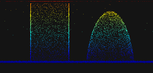
A point cloud is the “pixel” of the three-dimensional world, but it is far harder to handle than a two-dimensional image. A 2D image is a regular grid, where each pixel’s neighbors — which ones, how many — are fixed directly by its row and column indices; a point cloud, however, is a bag of unordered points, where who is adjacent to whom is nowhere written into the data structure and must be computed for yourself. It is sparse: outside the surface, the space holds no record at all. It is noisy: every point jitters along the measurement direction. And it has outliers: arc light, glare, and multipath conjure up a batch of “flyers” hanging in mid-air out of nothing. This chapter lays out all four of these properties in a single synthetic scene (Figure 37.1, Figure 37.2) and uses it to explain three of the most fundamental things: which forms three-dimensional data takes, how to find nearest neighbors fast on an unordered point set, and how to clean up the flyers.
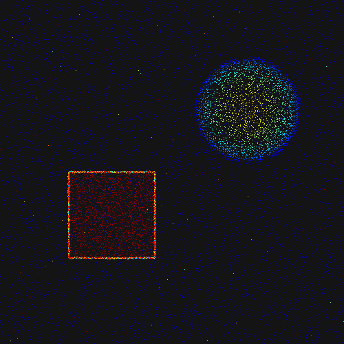
The whole scene comprises 20200 points: 11000 on the ground, 2600 on the cube top, 3600 on the four vertical sides, 2800 on the spherical cap, plus 200 outlier flyers. All surface points have Gaussian measurement noise of \(\sigma=0.10\) mm added along their respective normals, with a height range of \(z\in[-0.43,\ 43.92]\) mm (the surfaces themselves only reach 18 mm; everything higher is all flyers). This dataset is generated deterministically by the project in code/point_cloud_basics/ using a fixed random seed, and every number later in this chapter comes from its actual run.
37.1 Forms of Three-Dimensional Data
One and the same three-dimensional object can be recorded with three fundamentally different data structures, and in engineering you must keep them straight.
The first is the point cloud, the unordered point set \(\{\mathbf p_i=(x_i,y_i,z_i)\}\) mentioned above, optionally with a color or normal attached to each point. It is the most general form: it can represent surfaces of arbitrary topology, and multi-view stitching and free-form surfaces give it no trouble. The price is that it is unordered and irregular, so any “find the neighbors” operation must lean on an extra spatial index (the subject of the next section).
The second is the range image, also called a depth map or a 2.5D image. It is a regular two-dimensional grid, where each grid cell \((u,v)\) stores one height value \(z\) — essentially “an image that treats \(z\) as gray level.” Its biggest advantage is regularity: neighbor relations are given directly by the grid indices, all the filtering and morphology operators of two-dimensional images (Chapter 6) can be carried over and used unchanged, and storage is compact.
The third is the mesh, which explicitly records the connectivity of the surface with vertices plus triangular faces. It mainly serves rendering, finite-element analysis, and collision detection; it sees relatively little use in industrial measurement, so this chapter does not develop it.
The name “2.5D” pinpoints the awkward position of the range image: it has a complete \(x,y\) plane and a \(z\), looking three-dimensional, yet it stipulates that each \((x,y)\) can have only one \(z\). A true 3D surface, at a vertical wall, an overhanging face, or a cavity, lets a single line of sight pass through multiple \(z\) values, and that is exactly what a range image cannot express — it can only record “the nearest (or highest) layer seen from some fixed viewpoint.”
A point cloud and a range image can be converted into each other, but this conversion is not lossless. From range image to point cloud is simple: each valid grid cell is restored to a three-dimensional point according to its indices and height. The other way, generating a range image from a point cloud, first picks a projection direction (here we take the top view, looking along \(-z\)), bins the \(XY\) plane into a regular grid, and keeps only one representative \(z\) per bin. The problem lies precisely in this “keep only one.”
I binned these 20200 points onto a \(200\times200\) top-view grid, taking the highest \(z\) among the points falling into each bin, with the result in Figure 37.3: the gridding artifacts are plainly visible, the ground has been quantized into a mosaic, the spherical cap is still there, and the cube top is there too — but the cube’s vertical sidewalls have vanished entirely, and so has the ground directly beneath the cube and beneath the spherical cap, the part that was occluded. Statistically, of the original 20200 points, after reprojection only 12585 bins survive, losing 7615 points (37.7%). These lost points are not noise; they are real samples of a real surface, and they disappear purely because they share the same \((x,y)\) with other points whose \(z\) is higher — the sidewall points are covered by the top points, and the occluded ground points are covered by the object above.
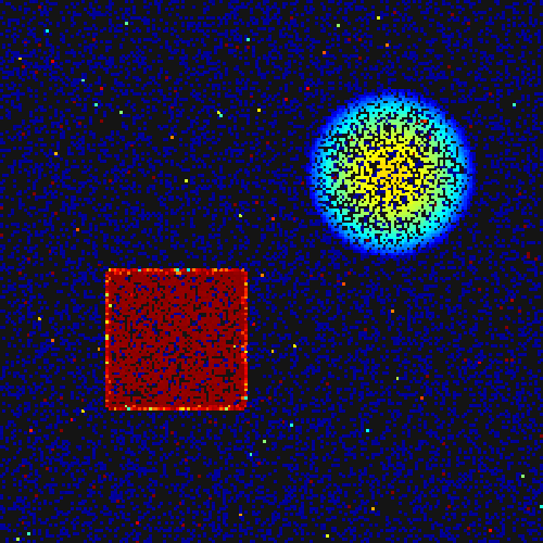
This 37.7% is not a number picked at random; it is a lesson on the “essence of a single viewpoint.” In Chapter 33, laser triangulation directly produces a range image, and at that point it naturally sees only the surface that can be illuminated from the laser’s viewpoint — the back, the sidewalls, and the cavities were in shadow from the start. The 2.5D limitation of the range image and the single-viewpoint limitation of the acquisition method are two ways of saying the same thing. To obtain a complete 3D you must either scan from multiple viewpoints and then register (Chapter 39), or simply work with point clouds the whole way and never collapse to a range image. So a practical engineering rule is: if you can use a point cloud, do not convert to a range image prematurely; only when you are sure that a single viewpoint suffices, and you want to borrow the mature operators of two-dimensional images, is the regularity of the range image worth trading away that 37.7% of information for.
In SciVision these two forms correspond, respectively, to SciPointCloud (points + optional color + optional normal, with PLY/PCD/OBJ read/write) and SciRangeImage (ushort height data plus resolutionX/Y/Z and offsetZ, stored as a 16-bit PNG). After this chapter’s scene is loaded into a SciPointCloud, Length=20200, and the saved cloud_raw.ply carries per-point height color and can be opened directly in any point-cloud viewer.
37.2 Spatial Indexing: KdTree
A point cloud is unordered, and the first, most fundamental engineering problem this brings is: given a query point, how do you find its nearest several neighbors? This “nearest neighbor query” is the bedrock of nearly all three-dimensional algorithms — registration relies on it to build point pairs (Chapter 39), filtering relies on it to define neighborhoods, and normal estimation, feature description, and surface reconstruction are no exceptions. The most naive approach is brute-force scanning: for each query point, compute its distance to all \(N\) points and then sort, \(O(N)\) per query, \(O(MN)\) for \(M\) of them. With \(N\) in the tens of thousands and \(M\) in the tens of thousands, this is tens of billions of distance computations — unacceptably slow.
The kd-tree brings this down to logarithmic complexity. Its idea is to recursively bisect space with hyperplanes perpendicular to the coordinate axes: at the root node, take the median along the \(x\) coordinate, send the smaller to the left subtree and the larger to the right; the next level switches to the \(y\) axis, the level below to the \(z\) axis, and so the cuts proceed with the axis rotating, until each leaf holds only a few points. Once built, a single nearest-neighbor query first descends to the leaf containing the query point (this leg needs only \(O(\log N)\) comparisons), obtains a batch of candidate neighbors, then backtracks upward: at each split node it checks whether “the distance from the query point to the splitting hyperplane” is still smaller than the current known \(k\)-th nearest — if not, the entire subtree on that side of the hyperplane cannot possibly contain a nearer point, and is pruned away wholesale, never to be entered. It is precisely this pruning that brings the average query complexity down to \(O(\log N)\). A \(k\)-nearest-neighbor query maintains the current nearest \(k\) with a max-heap of size \(k\); a radius search instead collects all points falling within a given radius, with the pruning criterion on backtracking switched from “the \(k\)-th nearest distance” to “the radius.”
The logarithmic complexity of the kd-tree has a precondition: the dimension must not be too high. When the dimension climbs to dozens or hundreds, “the distance to the hyperplane is almost always smaller than the distance to the nearest point,” the pruning almost entirely fails, and the kd-tree degenerates back to near-brute-force — this is the curse of dimensionality. Fortunately, a three-dimensional point cloud has only 3 dimensions, and the kd-tree is in its element here. High-dimensional feature matching turns instead to approximate nearest neighbors or locality-sensitive hashing.
This chapter’s project implements an implicit array-based kd-tree (using std::nth_element for the median split, with the axis rotating through \(x/y/z\)) and times it against brute force. For 20200 points doing 10000 queries of 8 nearest neighbors, the kd-tree takes about 60 ms, brute force about 870 ms, a speedup of about 14.5×; moreover the two results agree bit for bit — the kd-tree is not approximate and loses no precision; what it returns is exactly the nearest neighbors, only it cleverly avoids the impossible regions. This 14.5× shows little on a single query, but placed inside an iterative algorithm that queries nearest neighbors over and over (such as ICP, which every round finds correspondences for tens of thousands of points), it is the difference between a few minutes and tens of milliseconds — the engineering value of \(\log N\) versus \(N\) is cashed out precisely in such inner loops that are “called ten million times.”
37.3 Noise and Outliers
The “dirt” in three-dimensional data divides into two fundamentally different kinds, and lumping them together leads you to reach for the wrong tool.
The first kind is measurement noise: every real surface point has a small random jitter along the measurement direction (usually the surface normal), which in this chapter’s synthetic data is Gaussian noise of \(\sigma=0.10\) mm. Its hallmark is small amplitude, zero mean, hugging the surface — the points in a neighborhood are packed shoulder to shoulder, with uniform density. This kind of noise is handled by smoothing filters (later chapters of Part IX) and should not be dealt with by “deleting points.”
The second kind is outliers, that is, flyers: arc light, specular reflection, multipath, and sensor artifacts conjure up a batch of points that lie on no real surface at all, hanging in mid-air, far from all normal structure. This chapter’s 200 flyers are exactly so, sprinkled through the empty region \(z\in[6,44]\) mm. Their hallmark is just the opposite, far from the surface, with an empty neighborhood — a flyer has almost no other points around it, separated from its nearest neighbor by a large gap.
This “empty neighborhood” hallmark is exactly what can be used to pick out the flyers, and this is statistical outlier removal (SOR). The algorithm is naive to the point of being blunt: for each point, use the kd-tree to find its \(k\) nearest neighbors, and compute its average distance \(d_i\) to these \(k\) neighbors; normal surface points are packed together, so \(d_i\) is small, while a flyer hangs alone in the air, so \(d_i\) is large. Treat the \(\{d_i\}\) of all points as a distribution, find its mean \(\mu\) and standard deviation \(\sigma\), and judge every point with \(d_i>\mu+t\sigma\) to be an outlier and remove it. This is really the \(3\sigma\) rule from Chapter 2 applied to the quantity “neighborhood average distance,” and it shares its roots with the statistical anomaly judgment of Chapter 26 — rather than presetting a fixed distance threshold, it lets the data’s own distribution set the threshold.
Why should the threshold be set by the distribution rather than slapped down as a fixed number of millimeters? Because “how far counts as far” depends entirely on the density of the point cloud. The same 0.5 mm neighborhood-average distance is an outlier in a dense scan but normal in a sparse one. \(\mu+t\sigma\) hands the scale over to the data itself, so switching to a different point cloud requires no retuning of parameters — and this is exactly the robustness of a statistical threshold over a hard threshold.
This chapter takes \(k=8\), \(t=2\). On this data, the \(\mu+2\sigma\) of the neighborhood-average distance is \(3.23\) mm, by which 190 points are removed, of which all 190 hit true flyers (95% recall against the 200 flyers), with 0 false deletions — not a single real surface point wronged. Figure 37.4 marks the 190 removed points with red diamonds; they fall neatly in the empty region, exactly those floating flyers.
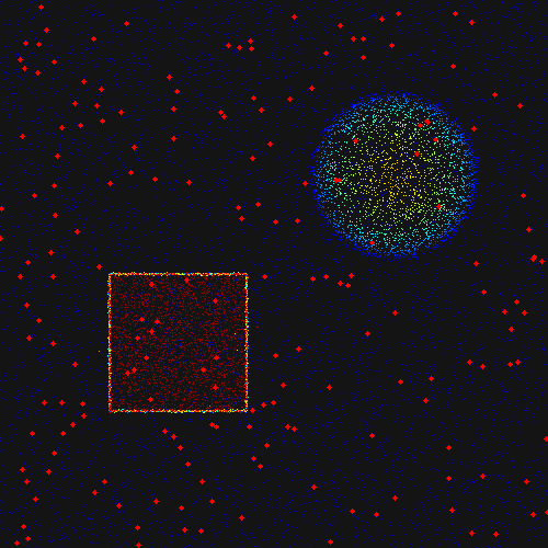
Where did the 10 missed flyers go? They were not removed because, unluckily (or rather too luckily), they happened to land near some real surface — if a flyer happens to drift very close above the ground or the cube, then real surface points slip in among its 8 nearest neighbors, its neighborhood-average distance is pulled down below the threshold, and it escapes the statistics. This is not a bug in the algorithm but an inherent boundary of the statistical method: SOR judges “neighborhood density anomaly,” and an outlier disguised as normal density it cannot tell apart. Being honest about these 10 escapees is more credible than reporting a 100% recall — downstream algorithms (such as robust fitting and ICP) ought to be resistant to the residual handful of outliers in the first place, rather than counting on the preprocessing to clean everything out in one pass.
37.4 SciVision Implementation
The I/O of the data forms is done with SciPointCloud, but there is a pitfall here that must be written down faithfully. SciPointCloud accepts a SciVector3dArray as its point set, and the constructor SciVector3dArray(float*, size) — the seemingly convenient “construct in one shot from a contiguous array” — is inert on this machine: after construction Length() is still 0, the points never went in at all. The reliable approach is to Append point by point:
SciVector3dArray pts;
for (int i = 0; i < n; ++i) {
    SciVector3d v(xyz[3*i], xyz[3*i+1], xyz[3*i+2]);
    pts.Append(v);              // append point by point; the float* constructor does not populate on this machine
}
pc.SetPoints(pts);             // pc.Length() = n thereafter
For nearest-neighbor queries, the SDK’s Sci3DKdTree is usable, and its results agree with the hand-written kd-tree:
SCIMV::Sci3DKdTree kt;
long rc = kt.CreateKdTree(pc);
SciVector3d q(xyz[0], xyz[1], xyz[2]);
int num = 0; SciVector3dArray pos; SciIntArray ind; SciFloatArray dist;
kt.FindKNearestNeighbors(q, 8, &num, &pos, &ind, &dist);
// first four entries of dist = 0.000 / 0.516 / 0.802 / 0.999, bit-identical to the hand-written kd-tree
The first neighbor distance is 0.000 (the query point found itself), and the rest match the hand-written implementation exactly, which gives us a cross-check: this chapter’s timing and SOR are both based on the hand-written kd-tree (for determinism and timability), and the SDK’s Sci3DKdTree serves as collateral evidence confirming correctness.
Data conversion SciSv3DDataConvert: the forward ConvertPointCloudToRangeImage (point cloud to range image) is usable, but the reverse ConvertRangeImageToPointCloud is inert on this machine (the surviving point count is 0), so the 2.5D loss experiment of Section 37.1 is done with hand-written binning, deterministic and controllable.
As for SOR, the SORFILTER feature of the SDK’s SciSv3DClean crashes on this machine (the measured exit code drifts with the heap layout; both 0xC0000005 access violation and 0xC0000409 stack guard have been seen). This chapter therefore uses a separate subprocess probe to poke at it (a crash will not drag down the main flow), while the real SOR uses a hand-written implementation:
// hand-written SOR: each point's average distance to its k-neighborhood, removed at the μ+2σ threshold
for (int i = 0; i < N; ++i) {
    kd.knn(&xyz[3*i], K+1, &nb);          // K+1: includes itself
    double sd = 0; int c = 0;
    for (auto& p : nb) {                  // skip itself, accumulate distances to K neighbors
        if (p.second == i) continue;
        sd += std::sqrt(p.first);
        if (++c == K) break;
    }
    meanD[i] = sd / c;                     // neighborhood-average distance d_i
}
double mu = /* mean(meanD) */, sigma = /* std(meanD) */;
double thr = mu + 2.0 * sigma;            // = 3.23 mm
for (int i = 0; i < N; ++i)
    if (meanD[i] > thr) removed.push_back(i);   // remove 190 points
This division of labor — “the SDK does I/O and cross-checking, the core algorithm is hand-written” — is the norm for the 3D modules of Part IX: point-cloud-class algorithms (kd-tree, SOR, ICP, PCA) are mostly self-contained and easy to write by hand, and the hand-written version further guarantees determinism and timability, whereas the maturity of the SDK’s 3D modules on this machine is uneven — use it where it works, isolate it where it crashes. The complete runnable project is in code/point_cloud_basics/.
Industry Case: A Flyer Storm in Laser-Scanned Point Clouds
Laser scanning of weld seams is a disaster zone for flyers. Arc light, spatter, and specular reflection off the base metal fill the sensor with spurious echoes, and flyers are dense; if you take such a point cloud straight to measure the weld reinforcement height or the undercut depth, the flyers pull the measurement datum off as a whole. The correct flow is to do SOR cleaning first, then measure, after which the weld contour immediately settles down. But SOR is a double-edged sword: set the threshold too strict, and it will falsely delete real thin edges and sharp features along with the flyers — the burr tip of a weld seam and the deepest point of an undercut are themselves neighborhood-sparse “lone points,” statistically looking much like flyers, and over-cleaning erases the very defect signal you set out to measure. The threshold must be set by the point cloud’s own noise distribution (\(\mu+t\sigma\) rather than a fixed number of millimeters). The rule: better to under-clean and hand the burden of outlier resistance to a downstream robust algorithm than to over-clean and throw away a real signal as noise.
37.5 Summary
- Three-dimensional data takes three forms: the point cloud is most general, the range image most regular, the mesh manages connectivity. The point cloud is an unordered point set that can represent arbitrary topology but needs an extra index; the range image is a regular 2.5D grid where two-dimensional operators apply directly, but each \((x,y)\) stores only one \(z\).
- Point cloud to range image is lossy, and the loss is proportional to the scene’s “verticality.” This chapter’s 20200 points reprojected onto a \(200\times200\) grid leave only 12585 (losing 37.7%), with the vertical sidewalls and occluded regions vanishing as whole swaths — this is the essential limitation of single-viewpoint 2.5D, echoing the single-viewpoint acquisition of laser triangulation. If you can use a point cloud, do not collapse to a range image prematurely.
- The kd-tree brings the nearest-neighbor query on an unordered point cloud from \(O(N)\) down to \(O(\log N)\): build the tree by axis-rotating median splits, and on backtracking prune by “distance to the hyperplane.” This chapter’s 10000 queries of 8-NN take about 60 ms for the kd-tree and about 870 ms for brute force, a 14.5× speedup with bit-for-bit exact results — the bedrock of every iterative 3D algorithm (registration, filtering, features).
- Three-dimensional “dirt” comes in two kinds with different remedies: measurement noise is small-amplitude, zero-mean, hugging the surface, handled by smoothing; outlier flyers are far from the surface with an empty neighborhood, handled by deleting points via statistical outlier removal (SOR). Do not lump the two together.
- SOR picks out flyers with a \(\mu+t\sigma\) threshold on the “neighborhood average distance,” with the threshold tracking the distribution: this chapter’s \(k=8\), \(\mu+2\sigma=3.23\) mm removes 190 points, hits true flyers at 95%, with 0 false deletions. The 10 that escaped landed near a surface, disguised as normal density — an inherent boundary of the statistical method, so downstream should retain robustness against residual outliers.
For a more systematic treatment of point-cloud data structures, spatial indexing, and three-dimensional filtering, read further in the book by Steger et al. (Steger, Ulrich, and Wiedemann 2018); for a quick reference on 3D geometry and range-image processing in a vision context, see (Szeliski 2022). The kd-tree spatial index originates in Bentley’s classic paper introducing the multidimensional binary search tree (Bentley 1975), which brings the nearest-neighbor query of this chapter from \(O(N)\) down to logarithmic time; and the point-cloud operators used here and in later chapters — voxel downsampling, statistical outlier removal, normal estimation — are in practice mostly referenced to the Point Cloud Library (PCL) implementation, surveyed by Rusu and Cousins (Rusu and Cousins 2011). The subsequent Chapter 38 and Chapter 39 will develop, respectively, three-dimensional filtering/downsampling and point-cloud registration.