22 Intensity, Color, and Gap Measurement
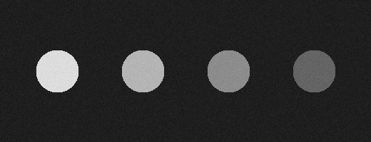
Not every measurement is about geometry. When an LED backlight panel comes off the line, the question is not “are the LEDs in place” but “are they bright enough, and is the brightness even”; for a batch of injection-molded housings, what must be checked is whether the color deviation from the reference swatch exceeds the limit; for a row of connector pins, the concern is whether adjacent gaps are consistent — any spot that is too wide or too narrow means a risk of poor mating. These three classes of problems fall under intensity measurement, color measurement, and pitch measurement respectively. The objects differ, but the skeleton is exactly the same: compute statistics inside an ROI → compare against the nominal value → judge by tolerance. This chapter walks through that pipeline with three actually-run experiments. Figure 22.1 is the scene of the first experiment: four LED spots, one of which is abnormally dim — but by eye alone, can you say for certain which one, and by how much?
22.1 Intensity Measurement
The essence of intensity measurement is computing statistics over the gray values inside an ROI. The most common statistics each have their role: the mean answers “is it bright overall,” and is the first choice for pass/fail judgments on brightness; the standard deviation answers “is it uniform inside,” useful for spotting local dead pixels or stains; the minimum/maximum/median characterize the two tails and the center of the distribution — the median is insensitive to a few outlier pixels and is more robust than the mean when the surface occasionally shows glints or dust. A single measurement call returns this whole set of statistics; take whichever you need.
The experimental scene is shown in Figure 22.1: four LED spots of radius 30 px with nominal intensities {220, 180, 220, 100}, where LED #2 is actually rendered at only 140 (simulating a dim-LED defect), and Gaussian noise of \(\sigma=4\) is added over the whole image. We place a circular ROI of radius 24 px at the center of each LED — deliberately one ring smaller than the spot, to keep the transition edge and the background out of the statistics. The SDK measures means of 220.11, 180.09, 139.97, and 100.06, with a maximum deviation from ground truth of only 0.11 gray levels; the measured standard deviations of 3.95-4.10 agree closely with the injected noise \(\sigma=4\). This shows that as long as the ROI is clean, the precision of gray-value statistics is limited almost solely by the noise itself — averaging over a thousand-plus pixels compresses the per-pixel \(\sigma=4\) random error down to the 0.1 level.
The standard error of the mean shrinks as \(\sigma/\sqrt{N}\): with about 1800 pixels in the ROI, \(4/\sqrt{1800}\approx 0.09\), consistent with the measured maximum deviation of 0.11. Measurement precision can be far better than single-pixel noise — this is exactly the value of statistical measurement.
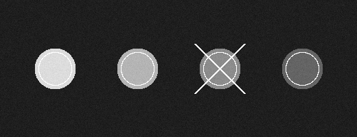
For the judgment step, we adopt the rule “a measured mean more than 40 gray levels below the nominal value is judged a dim LED.” The four LEDs have different nominal values, so the comparison must be made LED by LED against each one’s own nominal — not against a single global threshold: LED #2’s 140, compared against LED #3’s nominal 100, would actually look “bright.” The run flags exactly one LED — #2 — as DIM DEFECT (Figure 22.2). The tolerance of 40 is not pulled out of thin air: it should be anchored to the brightness variation the process allows (for example, the within-bin brightness spread after LED binning plus the drive-current tolerance), with additional margin for the measurement’s own uncertainty. Set the tolerance too tight and normal batch-to-batch variation gets falsely rejected; too loose and real defects slip through.
This experiment uses 8-bit images, with generous gray-level spacing between the 4 LED bins. If pass and fail for the object under test differ by only a few gray levels (e.g., transmittance grading of coated glass), the 256 levels of 8-bit quantization become the precision bottleneck, and 10/12-bit acquisition should be used instead (see Chapter 1).
One final reminder: intensity measurement measures “pixel gray value,” and pixel gray value = the object’s reflectance/emission characteristics × illumination × camera gain and exposure. The algorithm only cares about the first factor; any drift in the latter two passes straight into the measurement result. Illumination aging, voltage fluctuation, and ambient light leakage will all make the same panel measure different brightness at different times (Chapter 4). The robust practice on a production line is to fix an intensity reference patch inside the field of view: in every image, first measure the reference patch, then normalize the target reading by its value, canceling the illumination drift.
22.2 Color Measurement
The most direct way to extend intensity measurement to color images is to compute statistics on the R, G, and B channels separately. The experimental scene consists of four 80×80 color patches — blue, green, red, and orange-red — with noise of \(\sigma=5\) added per channel (Figure 22.3). Measuring a 64×64 rectangular ROI inside each patch, the three-channel means deviate from ground truth by at most 0.25, and the standard deviations deviate from \(\sigma=5\) by at most 0.12 — channel-level statistics are just as precise as in the grayscale case.

But “how much each channel differs” is not the same as “how different it looks to the human eye.” RGB space is perceptually non-uniform: the same Euclidean distance of 20 units is almost imperceptible in the green region yet jarring in skin tones. Industry’s standard language for color deviation is the color difference \(\Delta E\) in CIELAB space. CIE76 defines it as the Euclidean distance in Lab coordinates:
\[ \Delta E_{76} = \sqrt{(\Delta L^*)^2 + (\Delta a^*)^2 + (\Delta b^*)^2}, \]
The Lab space is constructed through a nonlinear transform so that equal \(\Delta E\) corresponds roughly to equal perceived difference. Empirically, \(\Delta E \approx 2.3\) is the just-noticeable difference (JND) — two colors closer than that cannot be told apart by an ordinary observer even side by side.
In the experiment, the BGR ground-truth values of the red and orange-red patches differ by only (5, 20, 5). Computed from the measured means: the BGR Euclidean distance is 21.02, and after conversion to Lab, CIE76 \(\Delta E = 5.85\) — about 2.5× the JND. This is precisely the typical regime of “close to the eye, separable by instrument”: picking these two swatches apart visually is a struggle, while a measurement system distinguishes them reliably and reports a continuous deviation. A note in passing: the SDK does not provide Lab output; the \(\Delta E\) here is converted in code via sRGB (D65 white point) → XYZ → Lab — see the companion project for the conversion formulas.
Division of labor between color measurement and color matching (Chapter 18): measurement answers “by how much it deviates,” outputting a continuous quantity, suited to quality grading and process monitoring; matching answers “which class it is,” outputting a category label, suited to sorting. The same production line often needs both.
In practice there are two SDK conventions you must know. First, with colorSpace=0, the mean/standard-deviation arrays returned by MeasureColor are ordered R, G, B — exactly the reverse of the image’s BGR storage order; treating index 0 as B will swap red and blue. Second, in the HSV output of colorSpace=2, hue is not the familiar 0-360 degrees or 0-180 (the OpenCV 8-bit convention) but degrees × 256/360, with a range of 0-256; pure red’s hue wraps around at 0 and 256, and the measured red patch returns 256.0 rather than 0. Hue-threshold judgments must handle this wraparound, or red targets will be missed wholesale.
22.3 Gap and Pitch Measurement
The representative third scenario is connectors, pin headers, and IC leads: large numbers of equally spaced repetitive structures, where the defect is typically that one of them is tilted, shifted, or missing. Setting up a caliper for each one (Chapter 20) certainly works, but a 64-pin connector would need 64 calipers — tedious and inefficient. The pitch measurer is the “batch caliper” designed for this scenario: within a scan band (band ROI), it extracts all edges matching the polarity convention along a single direction, pairs them as “rising edge - falling edge,” obtains each pin’s width and center from each pair, and subtracts adjacent centers to get the pitch sequence — measuring the whole row in a single call.
The experimental scene consists of 8 vertical bright pins (width 14 px, nominal center spacing 40 px), where pin #5 is shifted 3 px to the right as a whole to simulate a position defect, with \(\sigma=4\) noise added (Figure 22.4). The scan band spans all the pins, the direction runs left to right, and edge 1 takes black→white polarity (a pin’s left edge) while edge 2 takes white→black (the right edge).
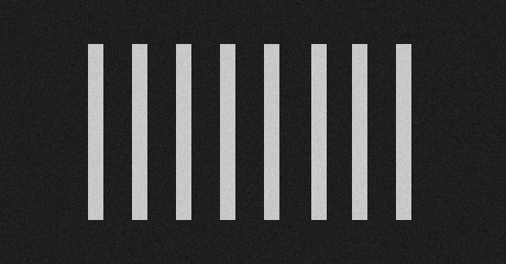
Measured results: the 8 pin widths come out at 13.98-14.03 (ground truth 14), with center localization error ≤0.01 px; the 7 pitches are, in order, 40.00, 40.02, 39.99, 40.01, 43.00, 37.00, 40.00. Judged against “nominal 40 ± 1.5 px,” exactly the two segments 4-5 and 5-6 are out of bounds, consistent with the SDK’s own outputs maxPitchIdx=4 and minPitchIdx=5. The result is shown in Figure 22.5.
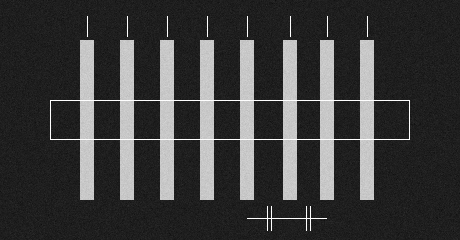
Note a pattern here that is worth committing to memory: one position defect shows up as two pitch anomalies. Pin #5 shifting 3 px to the right makes the pitch on its left become 43 and the one on its right 37 — one over-large segment immediately followed by an over-small one, with deviations equal in magnitude and opposite in sign. So when tracing a defect location back from the pitch sequence, do not report “segment 4-5 out of tolerance” and “segment 5-6 out of tolerance” as two separate defects; instead, find the common endpoint of the anomalous pair: pin #5, shared by both anomalous segments, is the true culprit. Conversely, if a single isolated pitch is anomalous while its neighbors are normal, the more likely cause is an abnormal pin width or an edge-extraction error — worth re-checking with a different criterion.
Pitch measurement shares the same subpixel edge kernel as the caliper — the ≤0.01 px center error in this experiment is of the same order as the single-edge localization precision in Chapter 20. The difference is only in scheduling: a caliper measures one edge pair at a time; the pitch measurer measures a whole row at once.
22.4 SciVision Implementation
The three classes of measurement are handled by SciSvIntensityMeasurement, SciSvColorMeasurement, and SciSvPitchMeasurer respectively. Intensity measurement:
SCIMV::SciSvIntensityMeasurement im;
SciROI roi;
SciPoint ctr(LED_CX[k], LED_CY);
roi.GenCircle(ctr, 24.0);                       // circular ROI, radius 24
double avg, sd, mn, mx, med, pixelTotal;
long rc = im.MeasureIntensity(img, roi, /*lower*/0, /*upper*/255,
                              NULL, &avg, &sd, &mn, &mx, &med,
                              NULL, &pixelTotal, NULL, NULL);
// pixelTotal: SDK output, measured 3324, not the ROI's geometric pixel count ~1810 — semantics unclear, do not use as an area in engineering
lower/upper are the gray-level gates for inclusion in the statistics (0..255 means all pixels) and can be used to exclude overexposed points; the outputs are, in order, mean, standard deviation, minimum, maximum, median, and pixelTotal (an SDK output, measured at 3324, which is not the ROI’s geometric pixel count of ~1810 — its semantics are unclear, so do not use it as an area in engineering); pass NULL for any output you do not need.
Color measurement (note that the two calls must use different ROI variables — the parameter is a non-const reference):
SCIMV::SciSvColorMeasurement cmeas;
SciROI roi;  roi.GenRect1(tl, br);               // GenRect1's bottom-right corner is an exclusive endpoint
SciVarArray avgRGB, stdRGB;
long rc = cmeas.MeasureColor(img, roi, /*colorSpace*/0,   // 0=RGB, 2=HSV
                             0, 255, 0, 255, 0, 255,      // per-channel statistics gates
                             /*model*/0, NULL, &avgRGB, &stdRGB, NULL, NULL);
double B = avgRGB[2].D(), G = avgRGB[1].D(), R = avgRGB[0].D();  // return order is R,G,B!
Pitch measurement:
SCIMV::SciSvPitchMeasurer pm;
SciROI band;  band.GenRect1(SciPoint(50,100), SciPoint(410,140));  // scan band spanning the pins
EdgeDirection dir;   // left to right; edge 1 black->white (left edge), edge 2 white->black (right edge)
dir.direction1 = 2; dir.direction2 = 2; dir.polarity1 = 0; dir.polarity2 = 1;
EdgeFilter filter;
filter.searchLineCount = 1; filter.edgeWidth = 2; filter.projectWidth = 2;
filter.sensitivity = 30; filter.strengthThresh = 5; filter.strengthLimit = 255;
double avgWidth, avgPitch;  SciVarArray widthArr, intervalArr, pitchArr, ang1, ang2;
SciPointArray edge1, edge2;  int maxW, minW, maxP, minP;
long rc = pm.PitchMeasurer(img, band, region, dir, /*pattern*/0, filter,
                           0, 0, /*widthThresh*/5.0, /*widthLimit*/30.0,
                           /*pairsCount*/8,
                           &avgWidth, &avgPitch, &widthArr, &intervalArr, &pitchArr,
                           &maxW, &minW, &maxP, &minP, &edge1, &ang1, &edge2, &ang2);
widthThresh/widthLimit bound the legal pin-width interval (5-30 px), filtering out noise edge pairs; pairsCount is the expected number of edge pairs; pitchArr returns \(N-1\) pitches, and maxP/minP directly give the indices of the largest and smallest pitch.
The pitfalls hit in practice are summarized below; all are handled in the companion project code/intensity_color_gap_measurement/:
MeasureColorreturns in R, G, B order, the reverse of the image’s BGR storage; values must be indexed in reverse;- HSV hue is degrees × 256/360 (0-256), with red wrapping around to 256.0; hue-interval judgments need wraparound handling;
PitchMeasurer’s edge-point arrays output 2 endpoints per edge (one each at the scan band’s top and bottom rims, interleaved): for 8 pins,edge1has length 16 rather than 8; when taking per-pin centers, first average the two endpoints of the same edge.
Industry Case: Backlight Luminance Uniformity
A backlight-module production line performed acceptance on uniformity with the 9-point method: 9 measurement points are taken across the screen, and the ratio of the dimmest point’s mean to the brightest point’s mean must be ≥80%. Single-point repeatability had always been good, yet customer complaints rose after mass production. Investigation found that the fixture’s metal clamping rim reflected light back onto the screen’s four corners, systematically inflating the means at the 4 corner points by about 5% — and the corners are precisely where a backlight is dimmest, so the inflated readings pushed the min/max ratio artificially high, and low-uniformity modules that should have been rejected were released. The fix came in two steps: add a light shield to the fixture to eliminate the reflection; and at the same time change each point’s statistic from the mean to the median, suppressing the pull of any residual glint on the readings. After the fix, the judgments once again agreed with visual evaluation. The lesson: the choice of statistic is part of the measurement design — the mean treats every pixel equally, while the median naturally discards a few outliers; when the environment at the measurement points cannot be controlled, the latter is often closer to “the brightness a person sees.”
22.5 Summary
- Three classes of non-geometric measurement share one skeleton: statistics inside an ROI → comparison against the nominal value → judgment by tolerance. The ROI must avoid edges and background; the tolerance must be anchored to process variation, not gut feeling.
- Statistics push precision below the noise: the standard error of the mean shrinks as \(\sigma/\sqrt{N}\) — in this chapter, the intensity-mean error is 0.11, the channel-mean error 0.25, and the pin-center error 0.01 px, all far below single-pixel noise.
- Color differences must be computed in a perceptually uniform space: RGB distance does not reflect visual difference; the industrial criterion is CIELAB \(\Delta E\), with JND ≈ 2.3; red vs. orange-red measured \(\Delta E = 5.85\) — close to the eye, separable by instrument.
- One position defect = two pitch anomalies: an adjacent anomalous pair in the pitch sequence, equal in magnitude and opposite in sign, points to its common endpoint; the pitch measurer is in essence a batched caliper.
- Remember three SDK conventions: color means return in R,G,B order, HSV hue is on the 256 scale and wraps around at red, and pitch measurement’s edge points output two endpoints (top and bottom) per edge.
For the radiometric and colorimetric foundations behind intensity and color measurement, and a systematic discussion of edge-pair measurement, see the book by Steger et al. (Steger, Ulrich, and Wiedemann 2018). The concepts of CIELAB, white point, and \(\Delta E\) used in this chapter trace to the authoritative colorimetry classic by Wyszecki and Stiles, where the definitions, data, and derivations of nearly every color space and color-difference formula are collected (Wyszecki and Stiles 2000). For brevity this chapter uses the CIE76 \(\Delta E\), whereas the shop floor more often uses the perceptually more uniform CIEDE2000; Sharma et al. give the complete implementation details, supplementary test data, and several mathematical observations for that formula, a practical reference for upgrading this section’s color-difference computation to the current standard formula (Sharma, Wu, and Dalal 2005).