40 3D Matching

ICP (Chapter 39) solves the problem of “pressing two already roughly aligned point clouds into subpixel agreement” — it is a refinement engine, but congenitally near-sighted: let the initial value be off by a few tens of degrees and it locks into the wrong local minimum, never to climb out again. Yet what the camera on a production line sees is never an isolated blob of points but a frame of cluttered scene: the ground, the bin walls, neighboring workpieces, noise — with the part to be found buried inside and its pose entirely unknown. 3D matching is responsible for precisely this “from nothing to something” step — locating a known model inside a cluttered scene point cloud and giving its rough 6 degrees of freedom (6DoF) pose, then handing this coarse pose off to ICP for refinement. It is the three-dimensional counterpart of 2D template matching (Chapter 16) and shape matching (Chapter 17), and the eyes of robotic grasping and assembly: only once the part’s “where and which way” is known can the arm even begin to reach for it.

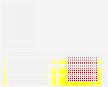
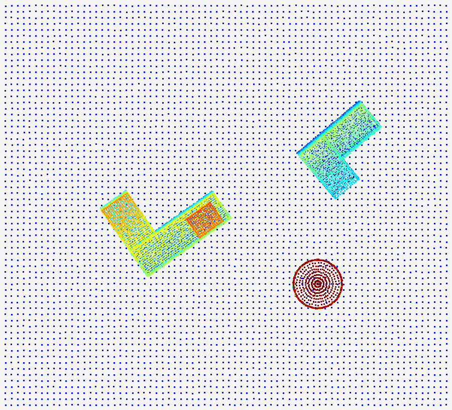
This chapter’s model is an asymmetric L-shaped bracket of about 5400 surface points: a long arm and a short arm form the L, with a boss added at the tip of the long arm (Figure 40.1 (a)) — the boss deliberately breaks the symmetry the L itself retains, making the principal-axis direction uniquely identifiable; the reason is in Section 40.2. The scene (Figure 40.1 (b)) contains two instances of this bracket, each at a different 6DoF pose: instance 1 clean and complete, instance 2 occluded (about 1/3 of the surface removed); in addition there is a ground plane and a distractor cylinder, with Gaussian noise of \(\sigma=0.1\,\text{mm}\) superimposed over the whole scene. The task is to find both instances and pin down their poses, while not mistaking the cylinder for the bracket.

(a) Model: the asymmetric L-shaped bracket template (height pseudocolor), long arm + short arm + top boss

40.1 Six-Degree-of-Freedom Pose Search

2D matching searches over three parameters \((x, y, \theta)\) — planar translation plus in-plane rotation; what let template/shape matching in the previous chapters score brute-force cell by cell over an angle × scale grid was precisely that the search space is only three-dimensional and that the image pyramid shrinks it level by level. Move to three dimensions and a rigid-body pose has 6 degrees of freedom: three translations \((t_x, t_y, t_z)\) plus three rotations (about the three axes). As the dimension rises from 3 to 6, the search space does not double but explodes exponentially — discretize each rotation axis into \(K\) steps and each translation axis into \(K\) steps, and the total number of candidates is \(K^6\). The motivation of Chapter 16 that “brute-force scoring cannot hold, a pyramid is mandatory” is, in 3D, magnified to the point of being unavoidable: even at a coarse \(30^\circ\)/\(10\,\text{mm}\) per axis, \(K\!\approx\!12\) already means millions of candidates, and each candidate still has to be scored by nearest neighbors over thousands of points.

The “6” of 6DoF is all the freedom a rigid body has in three-dimensional space: translation 3 + rotation 3. If the part may also scale (the working distance uncalibrated), add 1 more scale degree of freedom — but an industrial 3D camera is already calibrated to millimeters, the scale is usually fixed, and this is one thing 3D matching worries less about than 2D.

The conclusion is the same as in 2D, only more pressing: no brute force, coarse-to-fine is mandatory. First use cheap means to circle out the few candidates in the scene that “might be the part,” each with a coarse pose (coarse matching), then run ICP on only these few candidates to press the pose down to the noise floor (fine registration). Coarse matching is responsible for collapsing the \(K^6\) search into a handful of hypotheses, and fine matching for wiping out the few-degree, few-millimeter error of each hypothesis — neither can be spared, and this pipeline is the throughline of the chapter.

40.2 Coarse Matching Methods

The first step of coarse matching is not matching but scene segmentation: cutting a frame of point cloud into “individual candidate objects.” We reuse the two staples of point-cloud preprocessing (Chapter 38) — first fit the largest plane with RANSAC and strip away the ground (the ground is the plane with the most points in the scene; sample three points at random to fit, count inliers, and take the best over 200 iterations); once the ground is gone, the objects suspended above it separate from one another, and then comes Euclidean clustering: voxelize the space and, using a union-find structure, merge points in adjacent voxels whose distance is below a threshold (here \(4\,\text{mm}\)), so that each connected block is a cluster. After the ground is removed, this chapter’s scene splits cleanly into three clusters: the two bracket instances + one cylinder.

Each cluster demands a coarse pose. The most naive approach is principal component analysis (PCA): take the cluster’s centroid as the translation initial value, take the three eigenvectors of the covariance matrix as the object’s three principal axes, and align them with the model’s own principal axes to obtain the rotation initial value. The principle is plain — for a slender L-bracket, the point cloud’s direction of maximum variance must lie along the long arm, and PCA “sees” this axis at a glance. But PCA has two congenital limitations: first, the principal axes carry sign and ordering ambiguity — eigenvectors are arbitrary in sign, and under nearly equal eigenvalues the ordering can swing too, so all \(24\) right-handed combinations of the three axes are “equally reasonable” and must be tried one by one, disambiguated by “which one makes the model fit the scene best”; second, sensitivity to occlusion — delete part of the part and the variance distribution of the point cloud changes, the principal axes skew with it, and the rotation PCA gives can be off by tens or even hundreds of degrees. The latter is exactly the story of instance 2 (Section 40.3).

Beyond PCA there is a stronger class of coarse matching: the point-pair feature (PPF) — for pairs of points on the model, form a 4-dimensional feature from their distance and the angle between the two normals and vote out the pose; it is more robust to occlusion and clutter and is the cornerstone of Drost et al.’s industrial surface matching. This chapter uses PCA + multi-candidate search to demonstrate the principle; PPF takes considerably more implementation and is left as an extension.

This chapter generates all \(24\) PCA candidate poses for each cluster, runs a fast wide-capture-radius ICP on each, and picks the best by scene coverage (defined in the next section) — using one cheap “trial-and-error search” to make up for the fragility of PCA’s single estimate.

40.3 The Coarse-to-Fine Pipeline

This is the core teaching experiment of the chapter: coarse matching feeds the initial value, ICP presses down the noise floor, and the two instances play out both typical scripts of this pipeline in full.

Instance 1 (clean): with the surface complete and the point cloud dense, the PCA principal axes barely skew, and the winning candidate’s coarse pose is already at rotation error \(0.02^\circ\), translation error \(0.01\,\text{mm}\) — under full sampling PCA all but lands it in one step. After ICP takes over it is refined to \(0.01^\circ\)/\(0.00\,\text{mm}\), with inlier residual \(0.162\,\text{mm}\) and both scene coverage and model coverage reaching \(100\%\). Here ICP has almost nothing to do, because the coarse pose already sits near the noise floor.

Instance 2 (occluded): after about 1/3 of the surface is removed, the principal axes skew severely, and the best of the \(24\) candidates’ coarse poses is off by as much as rotation \(100.5^\circ\), translation \(21.8\,\text{mm}\) — taken on this number alone, PCA has all but failed. Yet it still places the model into the correct cluster, at the correct rough position, enough for ICP under a wide capture radius to progressively tighten the nearest neighbors and “twist” the model back bit by bit. In the end ICP converges to \(0.38^\circ\)/\(0.90\,\text{mm}\), residual \(0.400\,\text{mm}\). The reduction across the two stages is striking: rotation \(100.5^\circ\!\to\!0.38^\circ\) (about \(\times 266\)), translation \(21.8\!\to\!0.9\,\text{mm}\) (about \(\times 24\)).

The clean instance’s residual \(0.162\,\text{mm}\) falls right around the noise floor: for points with independent per-axis \(\sigma=0.1\,\text{mm}\), the RMS distance to the true surface is about \(\sigma\sqrt{3}\approx 0.17\,\text{mm}\). Once ICP converges to this order it is at the end of the line — any smaller would be overfitting the noise. The occluded instance’s \(0.40\,\text{mm}\) is slightly higher, the limit under partial data rather than an algorithm defect.

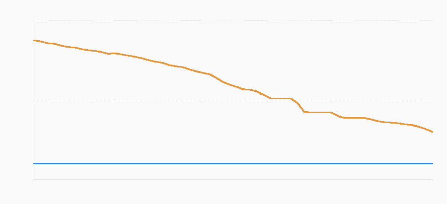
Figure 40.2 draws the two ICP convergence trajectories together (the vertical axis is residual on a \(\log\) scale). The orange line is the occluded instance: starting from the roughly \(4\,\text{mm}\) residual of the coarse pose, it steps down with the iterations to about \(0.4\,\text{mm}\) — each step the result of a tightened capture radius taking in more correct correspondences and shedding wrong ones. The blue line is the clean instance: pressed to the bottom from the start and nearly horizontal — it was at the noise floor all along, and ICP only confirms rather than carries. This figure is the closing footnote to Chapter 39’s assertion that “ICP needs a good initial value”: a good initial value (clean) leaves ICP nothing to do, a bad initial value (occluded) lets ICP show its worth, and a hopelessly bad initial value makes ICP fail outright — and this chapter, by “multi-candidate + wide radius,” rescues instance 2’s initial value to within ICP’s reach.

Figure 40.2: ICP convergence trajectories (horizontal axis iteration count, vertical axis inlier residual on \(\log\) scale, gridlines at \(0.1/1/10\,\text{mm}\)). Orange = occluded instance, stepping down from about \(4\,\text{mm}\) to about \(0.4\,\text{mm}\); blue = clean instance, hugging the noise floor (about \(0.16\,\text{mm}\)) almost horizontally throughout.

40.4 Occlusion and Coverage

In Chapter 17, 2D occlusion makes the score degrade by the visible fraction; 3D matching has to split “coverage” into two oppositely directed coverage measures, which measure different things.

Scene coverage: after placing the model at the candidate pose, how many points in the cluster land near the model surface. It asks “of this clump of points I found, how many can the model explain.” Occlusion only deletes scene points, and the remaining points still lie on the model, so scene coverage is insensitive to occlusion — and for exactly this reason it is chosen as the acceptance criterion: high coverage means accept this match.
Model coverage: conversely, how many of the model’s points found a corresponding scene point. The occluded portion of the part has no scene points to support it, so these model points go “unclaimed,” and model coverage drops directly with occlusion — which makes it just right for measuring how severe the occlusion is.

The experiment plays out their division of labor clearly. After occlusion removes about 1/3 of the surface: model coverage falls from the clean \(100\%\) to \(46.5\%\) (nearly halved, faithfully reflecting the amount of occlusion), while scene coverage drops only from \(100\%\) to \(79.3\%\) (still well above the acceptance threshold). In Figure 40.3 the blue occluded instance is visibly missing a stretch of geometry, yet its remaining points still seat snugly against the model — this is exactly the picture of “high scene coverage, low model coverage.” Were model coverage used as the acceptance criterion, the occluded instance would be wrongly rejected; with scene coverage, it passes smoothly.

The distractor cylinder is the counterexample: its geometry has nothing to do with the L-bracket, and however the model is placed, the cluster points never seat against the model surface — scene coverage is only about \(5.4\%\), far below the acceptance threshold, and it is cleanly rejected. The coverage criterion must both catch the genuine occluded part and block false targets of the wrong shape, and the cylinder is the touchstone for the latter.

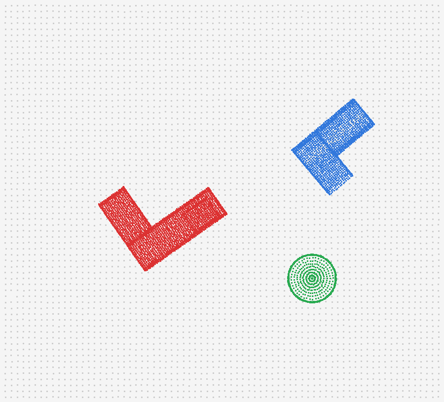
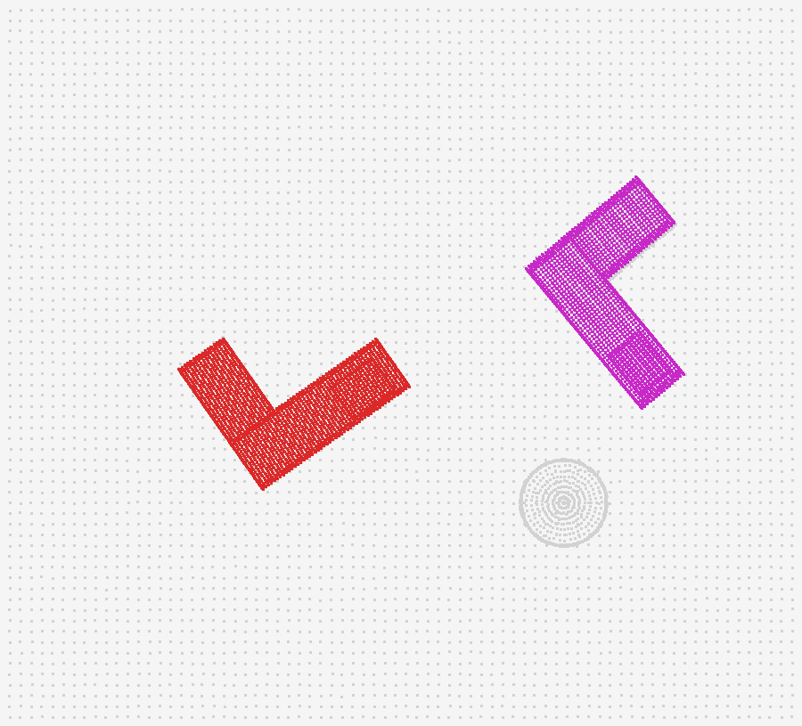
Figure 40.3: Scene segmentation result: gray = ground (already marked out by RANSAC), the three red/blue/green clusters being the Euclidean-clustering output — red the complete L, blue the occluded L (visibly missing a stretch of long-arm geometry), green the distractor cylinder.

Figure 40.4 is the final match: the model is overlaid back onto the scene at the two recovered poses, red at the clean instance and magenta at the occluded instance, both contours seating snugly; the cylinder, for want of coverage, is not overlaid. That the occluded instance can be localized successfully is the combined force of “PCA alone is not enough, naive ICP alone is not enough, the two in relay are enough” — which is of a piece with the logic of Chapter 17’s 2D shape matching that “the score degrades by the visible fraction, and minScore is the tolerable occlusion fraction,” only that 3D splits “one score” into “two coverages.”

Figure 40.4: Match result: the model is overlaid back onto the gray scene at the two recovered 6DoF poses, the clean instance red and the occluded instance magenta, both fitting; the distractor cylinder, for want of coverage, is not overlaid.

40.5 SciVision Implementation

As usual, first the honest record of what the SDK actually does in testing. SciVision provides two sets of 3D matching interfaces: SciSv3DSurfaceMatch (CreateSurface3DModel/FindSurface3DImageModel, range-image surface matching) and SciSv3DPointsMatching (GetTransformationICP/GetTransformationPCA, point-cloud registration). This chapter calls each via a subprocess probe, and both fail inertly: the return code is rc=0 (no error, no crash), but surface matching finds 0 matches and point-cloud ICP/PCA recovers a known translation as \((0,0,0)\), while the DLL also prints "Directory does not exist." to stderr — the same signature as several 3D modules in Part IX of this book (apparently a missing runtime resource directory). The SDK being unusable, the content of this chapter is carried by a hand-written pipeline.

The hand-written pipeline has four steps, with the key fragments below.

// 1) RANSAC ground removal: 200 random three-point plane fits, take the one with the most inliers
std::vector<char> ground = ransacPlane(scene, /*tol*/ 0.4);

// 2) Euclidean clustering: voxel + union-find, tol=4mm, discard clusters with <200 points
std::vector<std::vector<int>> clusters = cluster(rest, 4.0, 200);

// 3) Per cluster: PCA for centroid + principal axes, 24 signed-permutation candidates each run a
//    wide-radius fast ICP, pick the best by scene coverage (disambiguate + rescue skewed axes)
pca(clu, cs, Vs);                       // cluster centroid cs, principal axes Vs
for (auto& P : perms /*24 right-handed permutations*/) {
    matMul(Vs, P.data(), VsP); matMul(VsP, VmT, Rc);   // candidate rotation
    icp(modelScreen, clu, Rt, tt, 25, 14.0, 2.5);      // wide-capture-radius screening
    double sc = sceneCov(model, Rt, tt, cluDown, 0.6, rms);
    if (sc > bestSC) { /* record the best candidate */ }
}

// 4) Run a full ICP from the best candidate as initial value (Kabsch closed form, 3x3 SVD via Jacobi)
best.resid = icp(modelDown, clu, R, t, /*iters*/ 60, /*d0*/ 10.0, /*d1*/ 0.8);
best.sceneScore = sceneCov(model, best.R, best.t, cluDown, 0.5, rmsS);
best.ok = (best.sceneScore > 60.0 && best.resid < 1.5);   // coverage + residual dual criterion

Each ICP iteration finds the optimal rigid transform with Kabsch: de-mean the paired points, accumulate the covariance matrix \(C\), perform a Jacobi eigendecomposition on \(C^{\mathsf T}C\) to realize the \(3\times 3\) SVD, obtain the rotation from \(R=UV^{\mathsf T}\) (correcting for reflection so that \(\det R=+1\)), and find the translation from the difference of the two centroids. The capture radius tightens linearly from \(d_0\) to \(d_1\), which is exactly the source of the step-by-step descent of Figure 40.2’s orange line. The whole of the math is fully self-contained — which echoes Chapter 37 and a recurring observation of this book: point-cloud algorithms (ICP/Kabsch/PCA/PPF/kd-tree) mostly need to be self-developed or to lean on a dedicated library, and on 3D matching the SDK often serves only for IO and cross-validation. When industrial 3D matching is pushed to any depth, self-development is all but the norm.

40.6 Industry Case

Industry Case: Bin Picking of Randomly Stacked Parts

The same kind of part is randomly stacked in a bin (bin picking), and the arm must find each one’s pose and grab them off in turn. The 3D camera scans out a frame of point cloud, and the flow is the same as this chapter’s: remove the bin-bottom plane, Euclidean-cluster out the candidates one by one, and on each cluster solve a PCA coarse pose + ICP refinement. The difficulty lies in mutual occlusion in the stack — upper parts press on lower ones, most instances have very low model coverage, and accepting by model coverage would miss grasps wholesale. The countermeasure is exactly this chapter’s split of criteria: accept by scene coverage (occlusion-resistant), then sort by graspable-face visibility, grabbing first the one that is most complete and against which the gripper can seat steadily. Interference from the bin walls and neighboring parts is blocked by the coverage threshold — points of the wrong shape never seat against the model, the same way this chapter’s cylinder is rejected by its \(5.4\%\) coverage. The lesson distills to one line: the robustness of 3D matching = segmentation quality × coverage criterion, and the production rule under occlusion is “grab the one you can see most fully first.”

40.7 Summary

3D matching is the front end to ICP: ICP (Chapter 39) only refines and needs a good initial value; 3D matching locates a known model inside a cluttered scene and gives a coarse 6DoF pose to feed ICP. It is the three-dimensional counterpart of 2D template/shape matching (Chapter 16, Chapter 17).
Six degrees of freedom make brute-force search explode (\(K^6\)), so coarse-to-fine is mandatory: coarse matching (RANSAC ground removal + Euclidean clustering + PCA principal axes/centroid, \(24\) candidates for disambiguation) collapses the search into a handful of hypotheses, and ICP presses each hypothesis down to the noise floor.
The coarse-to-fine relay, measured: the clean instance is already near-fine from PCA (\(0.02^\circ\)/\(0.01\,\text{mm}\)), and ICP brings it to \(0.01^\circ\)/\(0.00\,\text{mm}\); the occluded instance’s coarse pose is off by \(100.5^\circ\), and a wide-radius ICP rescues it to \(0.38^\circ\)/\(0.90\,\text{mm}\) (rotation \(\times 266\), translation \(\times 24\)). PCA alone and naive ICP alone are both insufficient; only the relay suffices.
The division of labor between the two coverages: scene coverage (fraction of found points, occlusion-resistant) serves as the acceptance criterion, model coverage (fraction of the model explained) as the occlusion severity. Occlusion drives model coverage \(100\%\!\to\!46.5\%\) and scene coverage only \(100\%\!\to\!79.3\%\); the distractor cylinder is rejected at \(5.4\%\) scene coverage.
The honest SDK record: both SciSv3DSurfaceMatch and SciSv3DPointsMatching fail inertly (rc=0, zero matches / a recovered zero pose), and this chapter is carried by a hand-written pipeline (RANSAC + clustering + PCA + Kabsch ICP) — industrial 3D matching often needs self-development or a dedicated library.

The principles of 3D matching and the engineering practice of point-pair features and surface matching are treated systematically in the book by Steger et al. (Steger, Ulrich, and Wiedemann 2018). Encoding local geometry into a descriptor and then voting for the pose is the common thread of this family: Drost et al. use point-pair features (PPF) to model globally and match locally, a representative of industrial surface matching (Drost et al. 2010); earlier, Johnson and Hebert recognized 3D objects in cluttered scenes with spin images (Johnson and Hebert 1999); and the Fast Point Feature Histogram (FPFH) proposed by Rusu et al. is one of the most widely used descriptors for point-cloud coarse registration (Rusu, Blodow, and Beetz 2009), offering a more robust source of coarse pose beyond this chapter’s PCA.