14 Detecting Geometric Primitives

Place a part under the camera, and the first class of questions industrial vision must answer is often surprisingly plain: where is this edge? Where is the center of this hole? Alignment and placement close their motion loops on edge positions, dimensional inspection measures the distance between two edges, and robotic pick-up needs hole-center coordinates — in the end they all reduce to the same thing: locating points, lines, circles, and other geometric primitives in the image with subpixel accuracy. “Subpixel” is not a marketing word: in an imaging system at 10 μm/pixel, if localization is only accurate to whole pixels, the measurement resolution is nailed down at 10 μm; proper subpixel localization can reliably reach 1/10 pixel or better — equivalent to improving the system’s accuracy by an order of magnitude without changing a single piece of hardware.

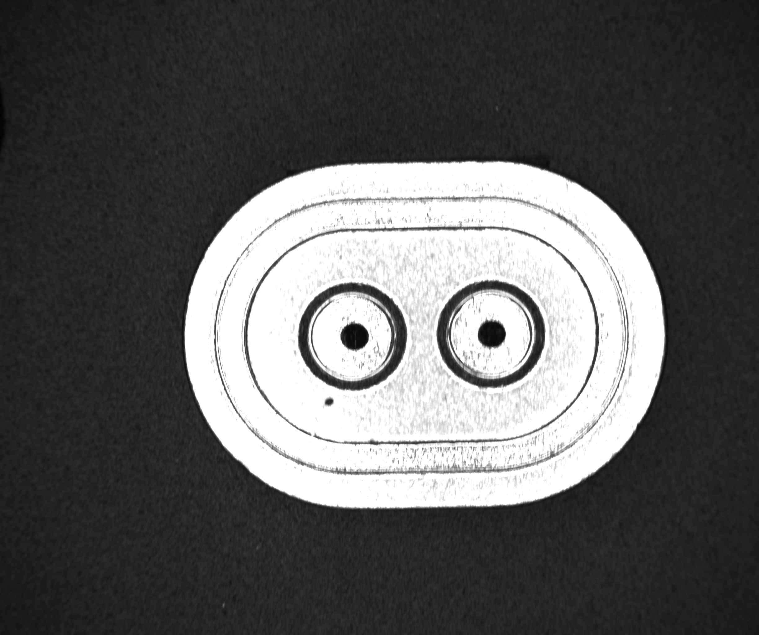
This chapter runs all of its experiments on one real industrial image (Figure 14.1): an oblong metal connector part on a dark background (2448×2048 single-channel grayscale, taken from Smart3’s standard “find point / find line / find circle” solution). The part’s outer contour has a roughly horizontal straight edge along the top — flat in the middle, rounding off at both ends — and inside it are two left-right symmetric bored holes, each with a circular bore mouth exposing the dark background at its center and a bright annular step around it. We will first extract a string of edge points along the top straight edge and fit a line to them, then cover each hole with a circular ROI and fit a circle — the rounded shoulders at the two ends of the straight edge will play the troublemakers, forcing out the full value of robust fitting.

Figure 14.1: The real test image: an oblong metal connector part on a dark background. The outer contour’s top edge is a roughly horizontal straight edge, flat in the middle and rounding off at both ends; inside the part are two left-right symmetric bored holes whose centers serve mating alignment and pick-up.

14.1 Extracting Edge Points

To locate an edge, you do not need to run edge detection over the whole image (that is the subject of Chapter 13). The industrial approach is far more direct: inside an ROI that roughly frames the target edge, lay down \(N\) mutually parallel search lines, splitting the two-dimensional localization problem into \(N\) one-dimensional ones. The processing along every search line is identical:

Take a gray profile: read the gray values point by point along the search line, yielding a one-dimensional curve.
Projection averaging: average over several pixels in the direction perpendicular to the search line (the projection within the projection width), using the average to suppress single-pixel noise — the same reasoning as in Chapter 6: independent zero-mean noise cancels under averaging.
First-derivative localization: take the first derivative of the averaged profile; an edge corresponds to an extremum of the derivative magnitude. Extrema whose magnitude falls below a threshold are treated as noise and not reported.
Subpixel interpolation: let the magnitudes at the discrete extremum of the derivative and at its left and right neighbors be \(g_0\), \(g_{-1}\), \(g_{+1}\); fit a parabola through these three points, and the offset of its vertex relative to the extremum is

\[ \delta = \frac{g_{-1}-g_{+1}}{2\,(g_{-1}-2g_0+g_{+1})}, \]

\(\delta\) falls within \(\pm 1/2\) pixel, and the subpixel edge position is “the whole-pixel extremum position \(+\ \delta\)”. Three samples determine one parabola, the vertex formula is closed-form, and the computational cost is negligible — subpixel accuracy is almost free.

This machinery comes with a set of parameters that can only be configured well if you understand the principle. The edge strength threshold (e.g. strengthThresh) is the admission gate on the first-derivative magnitude: set it too low and noise wiggles get counted as edges; too high, and genuine low-contrast edges are missed. Polarity specifies which kind of gray transition is accepted — black→white (rising), white→black (falling), or both: in this example we scan from top to bottom, crossing from the dark background into the bright part, a textbook black→white edge; locking the polarity immediately filters out half of the false edges. The edge width is the expected width of the gray transition band and determines the differencing span of the derivative: too small and it is noise-sensitive, too large and two adjacent edges get smeared into one. The projection width is a trade-off between noise suppression and blurring: the wider the projection, the more noise is averaged away and the more stable the edge strength estimate; but if the edge is not strictly perpendicular to the search line, too wide a projection “smears” the tilted edge sideways and the localization actually shifts — in practice 3 to 7 pixels is most common. The edge type decides which edge to report when a search line finds multiple candidates: the first, the last, or the one with the best strength; “best” is the most robust against weak false edges caused by oil stains and reflections.

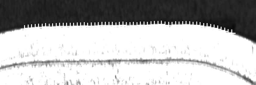
Figure 14.2 shows the extraction result with 60 search lines laid across the top-edge ROI: the ROI deliberately overruns the flat segment and reaches into the rounded shoulders at both ends, so among the 60 white crosses — the ones in the middle line up neatly along the true straight edge, while the ones at the two ends shift downward following the rounded corners. The search lines faithfully report the edge position they “see”, and that is how the shoulder points sneak into the point set (18 of them, by the criterion of distance \(|d|>5\) px to the fitted line). How not to be dragged off course by them is the subject of the next section.

Figure 14.2: Edge points extracted along the top by 60 search lines (white crosses). The middle ones line up along the true straight edge, while the points that overrun into the rounded shoulders shift downward following the contour, becoming the outliers in the subsequent fit.

14.2 Line Fitting: Least Squares and Robust Methods

With a string of edge points in hand, the next step is to estimate a line from them. Least squares (LSQ) fitting minimizes the sum of squared perpendicular distances from all points to the line

\[ \min_{L} \sum_{i} r_i^2, \qquad r_i = \operatorname{dist}(\mathbf p_i,\, L), \]

and the solution is closed-form (the line passes through the centroid of the point set, with its direction given by the principal eigenvector of the scatter matrix) — fast and free of hyperparameters. When all points are “roughly correct” it is optimal — the same statistical fact that makes averaging optimal under Gaussian noise. But it is extremely sensitive to outliers, and the reason hides in that square: residuals are squared before they are summed, so a shoulder point off by 30 px contributes 3600 times as much to the objective as a normal point off by 0.5 px. To appease a handful of large-residual points, the fitted line would rather rotate as a whole and let the majority of good points each be a little more wrong — the squared penalty being dominated by large residuals is the root cause of LSQ’s instability.

The idea of robust estimation is to replace the squared penalty with one that is more forgiving of large residuals. Huber’s scheme (Huber 1964) is equivalent to giving each point a weight that varies with its residual:

\[ w(r)=\begin{cases}1 & |r|\le \kappa\\[2pt] \kappa/|r| & |r|>\kappa\end{cases} \]

Points whose residual does not exceed the tuning constant \(\kappa\) enjoy a full say; points beyond it have their weight decay as \(\kappa/|r|\) — the larger the residual, the smaller the voice, but never a one-vote veto. Since the weights depend on the residuals and the residuals depend on the fit, the solution uses iteratively reweighted least squares (IRLS):

Input: edge point set {p_i}, tuning constant κ
1. Fit an initial line by ordinary least squares, all weights w_i ← 1
2. Repeat until convergence (line parameters change little enough,
   or the maximum number of iterations is reached):
   a. Compute each point's distance r_i to the current line
   b. Update weights by the Huber rule: if |r_i| ≤ κ then w_i ← 1,
      otherwise w_i ← κ/|r_i|
   c. Do a weighted least-squares fit with weights w_i, updating the line
3. Output the line and each point's final residual

In each iteration the outliers’ weights are pushed further down and the line steps closer to the “majority of good points”; convergence typically takes three to five rounds.

The other famous robust route is RANSAC (random sample consensus) (Fischler and Bolles 1981): repeatedly draw a minimal sample at random (a line needs only 2 points), fit it, count the “consensus” points falling within a tolerance band, and keep the model with the largest consensus. IRLS starts from all the points and converges by reweighting; RANSAC relies on random sampling to stumble upon an outlier-free sample. When the outlier fraction is very high (approaching or even exceeding half), RANSAC is more reliable; when outliers are few and the normal points carry continuous noise, IRLS is more accurate, faster, and its result is repeatable (no randomness) — industrial edge fitting mostly belongs to the latter case.

Talk is cheap, so let us run a controlled experiment on the 60 edge points from the previous section. The ROI overruns a stretch of rounded shoulder at each end, and the search lines falling into those stretches produce a small clutch of outliers shifted downward as a group (18 in total, three tenths of the 60 points). On the LSQ side, outlier rejection is deliberately switched off (rejectRatio=1, rejectDist=20 — a rejection threshold of 20 px lets every shoulder outlier participate in the fit); the Huber side uses rejectRatio=10, rejectDist=5. We evaluate both fitted lines under one uniform rule — the root-mean-square error (RMSE) over only the inliers whose distance to the respective fitted line satisfies \(|d|\le 5\) px: 2.793 px for LSQ, 1.456 px for Huber, nearly a twofold difference. Geometrically, the LSQ line is dragged down as a whole by the two shoulders and tilted by their asymmetric distribution, while the Huber line hugs the middle straight edge firmly.

A common evaluation trap: the RMSE returned by an SDK’s fitting interface is the all-point RMSE — 5.908 px on the LSQ side of this experiment, the bulk of which is the shoulder outliers’ own residuals. That number is unsuitable for comparing the accuracy of two fits: outliers have large residuals against any “correct” line, so all-point RMSE punishes the data, not the fit. A fair comparison must use a uniform inlier rule (such as \(|d|\le 5\) px in this example).

14.3 Fitting Circles and Ellipses

When locating a circular hole, the search lines switch from a parallel layout to a radial layout: cover the hole with a circular ROI and lay out search lines uniformly over angle, each scanning along the radial direction (from inside outward); everything else — projection averaging, first derivative, subpixel interpolation — is exactly the same as in the line case. The radial layout adds two key parameters: the expected radius expectRadius and the radius tolerance radiusRange, which constrain the search to an annular search band \([\,\text{expectRadius}-\text{radiusRange},\ \text{expectRadius}+\text{radiusRange}\,]\). In this example expectRadius=45 and radiusRange=30, giving a search band of 15–75 px. Constraining the search band wins twice: the bore mouth inside the hole and the annular step outside it are both excluded, so false edges drop sharply; and each search line’s scan length shrinks accordingly, saving time.

Circle fitting comes in two families, algebraic fitting and geometric fitting: the former minimizes the algebraic residual of the circle equation — closed-form and extremely fast, but its implicit weighting introduces bias; the latter minimizes the true Euclidean distance from each point to the circle — iterative but unbiased. The common practice in industrial libraries is to use the algebraic solution as the initial value and finish with geometric iteration, getting both speed and accuracy.

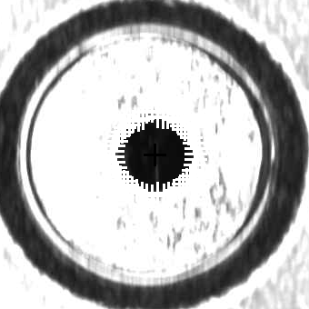
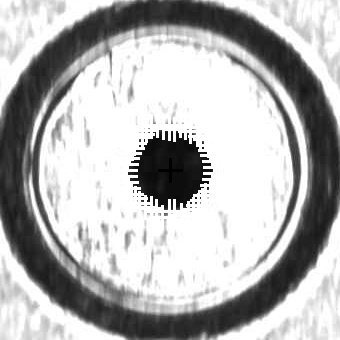
The experiment runs the circle finder once per hole: all 48 radial search lines hit the hole rim, yielding 48 edge points per hole (the white crosses in the two subfigures of Figure 14.3), with a black cross marking the fitted center. The left hole fits to center (1143.83, 1085.32), radius 44.60 px, the right hole to center (1586.00, 1077.59), radius 44.93 px, and the inter-hole center distance (pitch) is 442.06 px. All 48 edge points of each hole are effective points, with zero rejections — the part’s hole rims are intact, with no point deviating from the reference circle beyond the rejection threshold. The hole-center coordinates and the pitch are exactly the core quantities needed for connector mating and robotic pick-up: the pin-hole positions fix the pick target, the pitch locks the mating orientation.

(a) Left hole: 48 edge points (white crosses) + fitted center (black cross)

The robust fit hides one more “by-product” worth pointing out here: while delivering the reference circle, it also hands over a rejection list of “which points refuse to obey the reference.” On this part the hole rims are intact and the rejection list is empty; but the moment a rim develops a protruding burr, a chip-out, or boring-tool chatter marks, the corresponding edge points deviate from the reference circle and get screened out by the rejection threshold, and the position and clustering of the rejected points become markers of the defect directly. In other words, taking the fitted circle as the nominal contour and checking each edge point’s radial deviation, or the distribution of rejected points, accomplishes measurement and defect judgment in one and the same fit. Chapter 26 will develop this idea systematically.

14.4 SciVision Implementation

Edge-point extraction and line fitting are provided by SCIMV::SciSvLineLocator:

SCIMV::SciSvLineLocator lineLoc;
SciPointArray edgePts;
long rc = lineLoc.LinePointsLocator(src, lineROI, emptyRegion,
    /*strengthThresh*/ 25, /*direction top->bottom*/ 0, /*polarity black->white*/ 0,
    /*edgeWidth*/ 3, /*projectWidth*/ 5, /*edgeType best*/ 2,
    /*searchLineCount*/ 60, /*findPointType first derivative*/ 1, &edgePts);
rc = lineLoc.FitLine(edgePts, /*fitMethod Huber*/ 1, 10, 5, 0, 0, &lineHuber, &rmseHuber, &distHuber);

The parameters of LinePointsLocator map one-to-one onto the principles of Section 14.1: strengthThresh=25 is the gate on the first-derivative magnitude; direction=0 specifies scanning from top to bottom; polarity=0 accepts only black→white transitions (here we enter the bright part from the dark background); edgeWidth=3 and projectWidth=5 are the differencing span and the projection averaging width; edgeType=2 takes the candidate with the best strength; searchLineCount=60 search lines; findPointType=1 localizes by the first-derivative extremum. The output edgePts is the 60 subpixel edge points. In FitLine, fitMethod is 0 for least squares and 1 for Huber, and the following rejectRatio and rejectDist control outlier rejection during the fit (the number of rejection rounds and the distance threshold) — in the experiment of Section 14.2, the LSQ side used exactly the pair 1, 20 to effectively switch rejection off.

Circle finding is done in one step (search + fit) by SCIMV::SciSvEllipseLocator, called once per hole, reading the center and radius out of the output shape circleShape:

SCIMV::SciSvEllipseLocator circleLoc;
SciROI circleROI; SciPoint center(holeCx, holeCy);
circleROI.GenCircle(center, 80);   // circular ROI covering the rim search band
SciOverlay circleShape;
SciPointArray circlePts, circleEffect, circleReject;
rc = circleLoc.EllipseLocator(src, circleROI, emptyRegion, /*isEllipse*/ false,
    /*strengthThresh*/ 25, /*direction inside->outside*/ 0, /*polarity black->white*/ 0,
    /*edgeWidth*/ 3, /*projectWidth*/ 5, /*edgeType best*/ 2, /*fitMethod LSQ*/ 0,
    /*searchLineCount*/ 48, /*rejectRatio*/ 10, /*rejectDist*/ 5,
    /*expectRadius*/ 45, /*radiusRange*/ 30,
    &circleShape, &circlePts, &circleEffect, &circleReject);
SciPoint fc; double fr = 0; circleShape.GetCircle(&fc, &fr);   // hole center and radius

isEllipse=false means fitting a circle rather than an ellipse; direction=0 makes the search lines scan from the hole center outward; polarity=0 accepts only black→white transitions (crossing from the dark bore mouth into the bright step); fitMethod=0 is least-squares fitting, and rejectRatio=10 controls its outlier-rejection rounds; expectRadius=45 and radiusRange=30 delimit the 15–75 px annular search band (the circular ROI radius in this example is correspondingly set to 80). The four outputs are, in order: the fitted circle shape circleShape, all edge points circlePts, the effective points that participated in the fit circleEffect, and the rejected points circleReject — the two subfigures of Figure 14.3 plot each hole’s circlePts and fitted center. GetCircle extracts the hole’s center coordinates and radius from circleShape.

An honest disclosure: in the current SDK version, when fitMethod=1 (Huber), the RMSE output parameter of FitLine returns an invalid value (NaN). The companion project therefore uniformly computes the inlier RMSE itself from the array of point-to-line distances (the last output parameter of FitLine) — that is where the two numbers 2.793/1.456 in Section 14.2 come from. Commercial SDKs occasionally have such blemishes, and the engineering countermeasure is: recompute key metrics from the raw outputs (points, distances) wherever possible, instead of trusting summary values unconditionally. The complete runnable project that generates all of this chapter’s experimental images and numbers lives in code/geometric_primitives/, with its sample image self-contained at code/geometric_primitives/sample/connector.jpg.

Industry Case: Battery Electrode Edge Locating

The winding process in lithium battery manufacturing requires the anode and cathode electrode sheets to align with the separator to the 0.1 mm level, and the alignment loop depends on real-time locating of the electrode sheet edges. The difficulty is that slit electrode sheets almost universally carry burrs along their edges: with ordinary least-squares fitting, the burr points drag the edge line off, and the winding alignment inherits a systematic bias — robust fitting such as Huber (or piecewise local fits followed by a median) is mandatory to keep it down. The number of search lines is a direct trade-off between accuracy and cycle time: more lines, higher statistical accuracy of the fit, and linearly more time; production lines commonly use 30–100 lines, taking the upper end as the cycle-time margin allows. Another field-proven point is setting edgeType to “best edge”: oil stains on the electrode surface and reflections off the rollers create weaker false edges, so choosing “the first edge” easily locks onto the wrong target, while choosing the one with the best strength is essentially immune.

14.5 Summary

The standard industrial localization pipeline is “search-line sampling → 1D edge localization → subpixel interpolation → geometric fitting”: split the 2D problem into \(N\) 1D problems; on each search line, projection averaging suppresses noise, the first-derivative extremum pins the edge, and parabolic vertex interpolation yields the subpixel position.
Subpixel is almost free, but with preconditions: parabolic interpolation only delivers its accuracy when the profile is clean enough; the projection width (denoising vs. blurring), the edge strength threshold, the polarity, and the edge type must all be configured for the scene rather than left at defaults.
The root of least squares’ outlier sensitivity is the squared penalty: large residuals dominate the objective, and a handful of shoulder outliers is enough to drag the whole line off. Huber weighting + IRLS down-weights large-residual points by \(\kappa/|r|\); in this chapter’s experiment the inlier RMSE improved from 2.793 px to 1.456 px.
Comparing fitting accuracy requires a uniform inlier rule: all-point RMSE charges the outliers’ own residuals to the fit’s account — a common evaluation trap.
Robust circle fitting delivers measurement and defect clues in one pass: this chapter fits the center and radius of each of the two bored holes (a pitch of 442.06 px, directly usable for mating and pick-up), with zero rejected points on the intact rims; the moment a rim develops a defect, the rejection list becomes a position marker of it — the reference geometry serves measurement, the outlier list serves defect judgment.

For more accurate direct fitting of circles and ellipses, two classics on the algebraic solution are worth consulting: Taubin’s estimation of implicit curves and surfaces (Taubin 1991), and Fitzgibbon et al.’s ellipse-specific direct least-squares method (Fitzgibbon, Pilu, and Fisher 1999). For a more systematic treatment of subpixel edge extraction and geometric primitive fitting (including ellipses, circular arcs, and uncertainty analysis), see the book by Steger et al. (Steger, Ulrich, and Wiedemann 2018).