19 ROI Generation and Fixturing
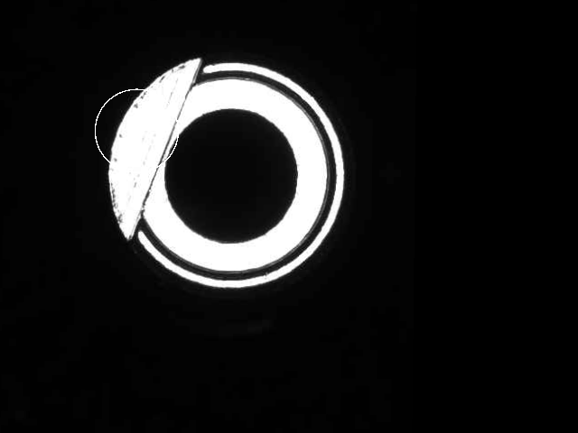
The previous chapters all solved the problem of “finding the part”: template matching (Chapter 16), shape matching (Chapter 17), and geometric primitive locating (Chapter 14) each work their own magic, but all ultimately hand over one position and one angle. On a production line, though, the real problem often only begins there — what happens after the part is found? A typical inspection station measures a dozen or even dozens of items on one part: hole diameters, edge distances, characters, defects… Every measurement item has its own ROI (region of interest), and the part arrives at a different position every time. Should every measurement item carry its own locating step? The standard answer on industrial lines is a far more elegant pattern: locate once, benefit everywhere — use a single locate to obtain the part’s current pose, then “carry” all the measurement ROIs to the part’s new position with one and the same transform. This mechanism is called fixturing. This chapter walks it through on a set of real sample images: the part under test is a rigid piece consisting of an illuminated ring plus a curved tab (Figure 19.1 (a), from the Smart3 “ROI correction sample recipe”), whose tab surface carries scratches and is precisely the object to inspect; Figure 19.1 (b) shows the same part moved elsewhere in the frame and rotated as a whole by about 90°. The white cross is the located ring center, and the thin line points to the tab. The inspection ROI (white circle) sits on the tab in the reference image — all the work ahead amounts to making that circular ROI catch up with the tab, which has moved 234 px.
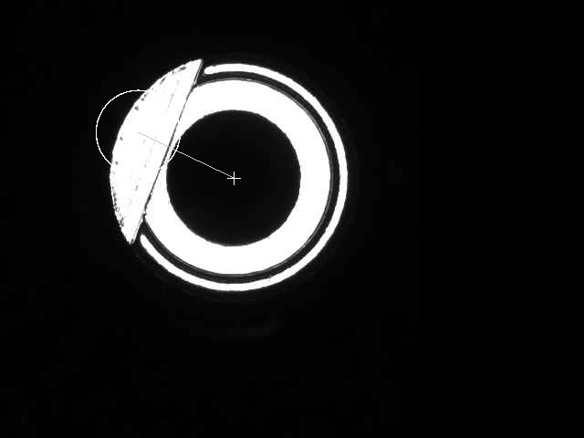
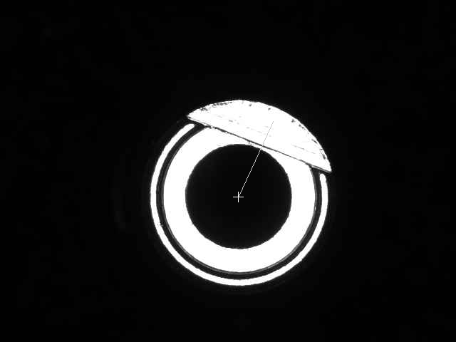
This sample set contains 7 images, all the same rigid part imaged at different incoming poses: the ring’s inner-hole radius is stable at 74.0 px across all 7, the distance from the tab centroid to the ring center is stable at 116 px, and the bright-pixel count is constant at about 29565 — these invariants are the fingerprint of “one and the same rigid body”. The part appears in three orientations: 001/006 (tab at upper left; the two are in fact a duplicate of the same image), 002–005 (tab rotated to the upper right; the four are pure translations of each other), and 007 (tab rotated to the lower left).
19.1 ROI Types and Generation
ROIs have appeared again and again in the preceding chapters; here is a systematic inventory. SciVision’s SciROI generates the various shapes through a family of Gen* methods: the rectangle (GenRect1, axis-aligned) is the most general — thresholding, filtering, and almost every other region operation uses it; the rotated rectangle frames tilted edges or character lines; the circle (GenCircle) naturally matches circular features such as holes, shafts, and solder joints, and this chapter’s inspection ROI is a circle sitting on the tab — the radial search lines of Chapter 14 are likewise laid out inside a circular ROI; the torus (GenTorus) constrains the search band between an inner and an outer radius, exactly right for measuring sealing rings and gaskets; the polygon hugs irregular contours. One engineering fact is worth recalling: the bottom-right corner of GenRect1 is an exclusive endpoint — a full-image ROI should be passed as (W, H) rather than (W−1, H−1), or the outermost row and column will go unprocessed (Chapter 7).
Since the ROI must move with the part, one has to ask: what does each ROI type become under a rigid transform? The center moves, the radius stays — a circle remains a circle, and this chapter’s circular inspection ROI is still a circle after a fixturing with an angle (measured below); the same goes for the torus. An axis-aligned rectangle, once rotated, is no longer axis-aligned — it becomes a rotated rectangle, which is exactly why rotated-rectangle ROIs are everywhere in fixturing pipelines: the upright rectangles drawn casually on the reference image all acquire an orientation after one fixturing with an angle. A polygon transforms vertex by vertex, its shape unchanged. In other words, all of these ROI types are closed under rigid transforms (under an affine transform a circle would become an ellipse, but fixturing never needs a transform that general), so there is no geometric obstacle whatsoever to ROIs following the part.
An ROI has two identities, and beginners often see only the first. The first identity is bounding the computation: a 640×480 image has three hundred thousand pixels, while a circular ROI of radius 46 around the tab has fewer than seven thousand — the algorithm runs only inside the ROI, a one-to-two-orders-of-magnitude difference in speed. The second identity matters more: the ROI binds the measurement semantics — “inside this circular ROI there should be the tab, and we are checking its surface for scratches”. The algorithm’s parameters (expected grey level, polarity, thresholds) are all configured according to “what is inside the ROI”; once the ROI no longer covers the feature it is supposed to cover, those parameters lose their premise entirely, and the algorithm either fails or — more dangerously — computes a plausible-looking result on the wrong content. This chapter’s experiment demonstrates the latter case on purpose.
19.2 Pose and the Rigid Transform
A pose is the union of “position + orientation”: the pose of a rigid planar part is fully determined by three quantities, the coordinates of a base point \(\mathbf{p}=(x, y)\) and an angle \(\theta\). The base point can be the template origin reported by a matching algorithm, or, as in this chapter, the center of a circular feature; the angle is taken along some directional reference. This chapter uses the center of the ring’s inner hole as the base point (the translation origin) and the direction from that center to the tab centroid as the angle — the center supplies the translation, the tab supplies the rotation, and together they lock down the pose of the whole part. Let a point \(\mathbf{f}\) in the part’s local coordinate frame (say the tab centroid) have an image position determined by the pose:
\[ \mathbf{x} = R(\theta)\,\mathbf{f} + \mathbf{p}, \qquad R(\theta)=\begin{bmatrix}\cos\theta & -\sin\theta\\ \sin\theta & \cos\theta\end{bmatrix}. \]
The reference pose \((\mathbf{p}_r, \theta_r)\) and the current pose \((\mathbf{p}_c, \theta_c)\) give the same point two image coordinates \(\mathbf{x}_r\) and \(\mathbf{x}_c\); eliminating \(\mathbf{f}\) yields the rigid transform from reference image coordinates to current image coordinates:
\[ \mathbf{x}_c = R(\Delta\theta)\,(\mathbf{x}_r - \mathbf{p}_r) + \mathbf{p}_c, \qquad \Delta\theta = \theta_c - \theta_r. \]
Written as a homogeneous matrix this is the familiar \(3\times 3\) form from Chapter 2: a rotation part \(R(\Delta\theta)\) and a translation part \(\mathbf{p}_c - R(\Delta\theta)\,\mathbf{p}_r\). The entire mathematics of fixturing is this single matrix: it holds for any point on the reference image, so one locate can drive arbitrarily many ROIs.
Hidden here is a very practical property, one that this chapter’s “coarse” angle estimate happens to confirm. Our angle does not come from a high-precision edge fit; it is the centroid direction of the bright pixels in the tab region — an estimator with a systematic bias that can be pulled off by several degrees by uneven illumination or the distribution of scratches. But as long as this bias is approximately constant in the part frame (same tab, same imaging), write it as \(\hat{\mathbf{p}} = \mathbf{p} + R(\theta)\,\mathbf{b}\) and substitute into the relative transform, expanding about a true feature point \(\mathbf{x}_r = R(\theta_r)\mathbf{f}+\mathbf{p}_r\) on the reference image:
\[ R(\Delta\theta)\,(\mathbf{x}_r - \hat{\mathbf{p}}_r) + \hat{\mathbf{p}}_c = R(\theta_c)\,\mathbf{f} - R(\theta_c)\,\mathbf{b} + \mathbf{p}_c + R(\theta_c)\,\mathbf{b} = \mathbf{x}_c . \]
The two \(R(\theta_c)\,\mathbf{b}\) terms cancel exactly — as long as the bias moves with the part, it has no effect on the fixturing whatsoever. The experiment bears this out: even though the angle estimate itself is a coarse centroid direction, because the reference and current images use the same estimator, the residual between the fixtured ROI center and the independently measured tab centroid stays \(\le\) 0.27 px throughout (worst case sample 004, 0.266 px). This is fixturing’s most easily overlooked teaching point: fixturing uses a relative transform, so a systematic bias in the locating feature is “wrong by the same amount on both sides” and cancels on subtraction; what truly eats precision is the random jitter of the angle and the part’s own non-rigidity.
The word “fixturing” comes from the machining fixture: a fixture locks the workpiece into a fixed pose so the tool path need not sense the workpiece. Visual fixturing does the opposite — the workpiece is placed freely, and the “tool path” (the ROI) adapts to the workpiece, amounting to a software fixture.
The cancellation presumes the bias is constant in the part frame. If the bias comes from factors in the image frame such as illumination direction or lens distortion, it does not rotate with the part and will not cancel — one reason the locating feature should be a high-contrast, well-isotropic structure (such as this chapter’s illuminated inner hole).
19.3 The Fixturing Experiment
The complete chain has four steps: locate → compute the fixturing matrix → transform the ROI → measure. Locating splits into two branches: the ring center is found from the inner-hole edge — scanning radially over angles to find the dark→bright transition gives the inner-hole edge points, and a least-squares circle fit on them converges the inner-hole radius to 74.0 px on all 7 images; the angle is then taken as the direction from the center toward the tab centroid (the centroid of bright pixels at radii in [134, 210]). Note that the locating extent and the measurement ROI play different roles: locating scans the large-scale structure of the whole part (a ring over a hundred pixels across), large enough to lock the part at any incoming position; the inspection ROI is the small, accurate one that must be carried by fixturing. With sample 001 as the reference, the locate result is ring center (255.56, 194.54) and tab direction −154.5°; the inspection ROI is then defined on the tab centroid (150.93, 144.67) measured on the reference image (a circle of radius 46) — fixturing carries “the position seen on the reference image”, so keeping the ROI definition consistent with the locate result is the engineering convention.
We initially tried SciVision’s SciSvEllipseLocator to fit the inner-hole circle, but it selects edges unstably on this sample set: it returns 123501012 outright on 001/006, and on 002–005 it locks onto the outer-ring edge (radius about 87 px) rather than the inner hole (74 px), with the center off by about 24 px. A center inconsistent from image to image would utterly corrupt the relative pose, so we switched to a deterministic “radial edge + circle fit”, whose inner-hole radius is stable at 74.0 px across the whole set.
The second step hands the two poses to SciAxisTransform::Generate2DAlignMatrix, yielding the \(3\times 3\) fixturing matrix from the reference pose to the current pose. Compared element by element with the rigid matrix computed by hand from the previous section’s formula, the maximum difference is below \(10^{-3}\) — what the SDK does is exactly that mathematics. A self-check with TransformPointAndAngle follows: pass the reference center through the matrix, and the residual to the current center is 0.0000 px, fully consistent.
The third step, AlignROI, transforms the inspection ROI (the radius-46 px circle hung on the tab in the reference image) to the current pose. A rigid transform does not change the shape, so a circular ROI stays a circle after transformation. Running this pipeline over all 7 samples, the recovered poses and alignment residuals are listed in Table 19.1: 002–005 are rotations of about +90° about the reference plus various translations, 007 is about −90°, and 006 coincides with 001 (the duplicate image, recovered as the identity transform). For every image the fixtured ROI center agrees with the independently measured tab centroid down to sub-pixel — the worst residual is only 0.266 px.
| Sample | Recovered translation (px) | Recovered rotation \(\Delta\theta\) | ROI→tab residual | Bright-pixel fraction (fixtured/unfixtured) |
|---|---|---|---|---|
| 001 | (0.0, 0.0) | 0.00° | 0.000 px | 0.718 / 0.718 |
| 002 | (+78.9, +81.0) | +89.36° | 0.164 px | 0.718 / 0.000 |
| 003 | (+128.9, +81.0) | +89.84° | 0.097 px | 0.718 / 0.000 |
| 004 | (+128.9, +131.0) | +89.73° | 0.266 px | 0.718 / 0.000 |
| 005 | (+128.9, −19.0) | +89.80° | 0.202 px | 0.719 / 0.000 |
| 006 | (0.0, 0.0) | 0.00° | 0.000 px | 0.718 / 0.718 |
| 007 | (−51.0, −21.1) | −89.81° | 0.119 px | 0.720 / 0.388 |
The core comparison is in the last column. Take sample 002: the tab moved 234 px from its reference position; after fixturing the circular ROI has a bright-pixel fraction of 0.718 (the tab fills the ROI), whereas the ROI left in place has a bright-pixel fraction of 0.000 — it lands on the pitch-black background in the upper-left of the frame, not covering a single illuminated pixel. Figure 19.2 compares the two visually.
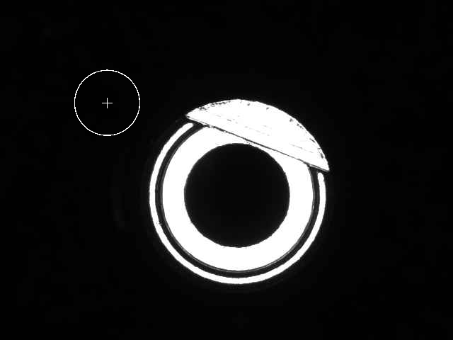
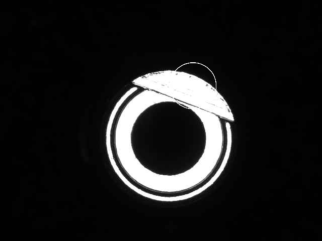
The fourth step runs the inspection inside the fixtured ROI — this chapter uses the “bright-pixel fraction” as the observable for whether the tab is in place (a real line would inspect for scratches or measure the contour inside this ROI): the fixtured ROI gives 0.718, exactly matching the 0.718 of the same ROI on the reference image, so fixturing eats essentially none of the inspection budget.
What truly warrants caution is the result on the unfixtured side. Intuitively, with the ROI off by over two hundred pixels, the inspection should simply fail and raise an alarm; but if the inspection algorithm only checks the return code, it will return normally on that black background — bright-pixel fraction 0.000, “no scratch found”, a seemingly perfect pass. This is the classic silent failure: the pipeline raises no error, the fields are filled in, yet the values were computed on the wrong content. It is far more dangerous than an outright error — an error stops the line, while a silent pass lets a bad part through. The engineering countermeasure is to guard the measurement with structural thresholds: the amount of valid signal inside the ROI (e.g. a bright-pixel fraction that is too low), whether the feature exists at all, the deviation from an expected model — any one out of bounds marks the measurement invalid, never trusting the return code alone. Here the gulf between 0.000 and 0.718 is a ready-made criterion.
19.4 Two Routes: Move the ROI or Move the Image
Fixturing has a second route, also the “tempting wrong turn” discussed in Chapter 10: instead of moving the ROI, transform the entire current image back to the reference pose by the inverse of the fixturing matrix, then measure with the original ROI as usual. This chapter implements that route with a hand-written bilinear inverse mapping (the same as the hand-written rotation of Chapter 10); the result is Figure 19.3: after sample 002 is rotated back, the part nearly reproduces the layout of reference image 001, and the original ROI again sits on the tab.
The two routes give almost equal bright-pixel fractions inside the fixtured ROI: moving the ROI gives 0.718, rotating the image gives 0.722 — mathematically they are the same transform, the difference being only interpolation noise (0.004). But the cost is wholly unequal: moving the ROI transforms only a few geometric parameters (two numbers for the center, one for the radius), at negligible cost; moving the image resamples all three hundred thousand pixels once, and bilinear interpolation lays a layer of smoothing over the edges, degrading the repeatability of edge localization (the case in Chapter 10 quantified this degradation). The conclusion matches that chapter: if you can move the ROI, do not move the image. Moving the image is worthwhile only in two situations: the algorithm accepts only axis-aligned ROIs and cannot express an oriented inspection region; or several stations and several algorithms must share one reference coordinate frame, where a single unified rotation is more controllable than each stage fixturing on its own.
19.5 SciVision Implementation
The heart of fixturing is two interfaces of SciAxisTransform:
SCIMV::SciAxisTransform xform;
SciMatrix M;
SciPoint refPt(poseRef.cx, poseRef.cy), curPt(poseCur.cx, poseCur.cy);
long rc = xform.Generate2DAlignMatrix(refPt, curPt,
    (float)(-poseRef.deg), (float)(-poseCur.deg), &M);   // negate the angles, see below

SciROI fixedROI;
rc = xform.AlignROI(inspROI, M, &fixedROI);              // a circular ROI stays a circle
The four inputs to Generate2DAlignMatrix are, in order, the reference base point refPt, the current base point curPt, the reference angle, and the current angle; it outputs the \(3\times 3\) matrix M from the reference pose to the current pose. AlignROI passes any SciROI through the matrix to obtain the fixtured ROI. To verify the matrix is correct, use TransformPointAndAngle, which transforms a point and an angle together, well suited to the self-check “the reference center should land on the current center”.
This chapter hit two pitfalls on real samples; both are recorded faithfully. The first pitfall most deserves underlining: the sign of the angle. Generate2DAlignMatrix adopts the convention visual counter-clockwise is positive; but the pixel coordinate system has the y axis pointing down, so the angle computed by atan2(dy, dx) is positive clockwise in the visual sense — the two differ by a sign. Pass the atan2 result straight in and the rotation direction reverses, sending the fixtured ROI off by hundreds of pixels, worse than no fixturing at all. The correct practice is to pass -poseRef.deg and -poseCur.deg. The handedness issue of coordinate frames was emphasized in Chapter 2; this is its most painful appearance.
The second pitfall is in the locating step: SciSvEllipseLocator selects edges unstably on this set of illuminated-ring samples — it returns 123501012 outright on two of the images, and on the other four it locks onto the outer-ring edge (radius about 87 px) instead of the target inner hole (74 px), with the center off by about 24 px. Fixturing consumes the difference of two locates, so once the locating source drifts and loses self-consistency from image to image, even the most accurate matrix is fed garbage input. This chapter therefore switched to a deterministic “radial dark→bright edge points + least-squares circle fit” for the inner-hole center, and all 7 images converge to the same radius 74.0 px, which is what makes self-consistency possible. This lesson outweighs any single-point accuracy: the precision ceiling of a fixturing system is set by the repeatability of locating, not by the absolute accuracy of a single frame. The complete project that produces all figures and numbers in this chapter is at code/roi_and_fixturing/.
Industry Case: Many Measurements Share One Locate
A connector inspection station had 23 measurement items: pin pitch, plastic-shell edge distance, latch contour… At first each item ran its own template-matching locate, badly overrunning the cycle time, and because each item’s locating error was independent, cross-item dimensions like “pin to shell edge” jittered noticeably. The redesign located the whole connector once by shape matching and transformed all 23 measurement ROIs through one and the same fixturing matrix: cycle time dropped by about 60%, and more importantly all items shared one coordinate datum — the relations among items were no longer polluted by their individual locating errors. The price is that locating quality becomes a global single point of dependency: once locating fails or drifts, all 23 items go down together. This is exactly the lesson this chapter’s samples teach — the repeatability of locating is the lifeline of a fixturing system. In deployment a score threshold and failure retries (changing parameters, changing the search region) were added to locating, and the trend of the locating score across product batches was brought into monitoring.
19.6 Summary
- The standard pattern of fixturing is “locate once, benefit everywhere”: one locate gives the current pose, and one rigid-transform matrix drives all measurement ROIs to follow the part — across this chapter’s 7 real samples, the residual between the fixtured ROI and the tab is everywhere \(\le\) 0.27 px, while the unfixtured ROI misses outright (the tab moved 234 px, and the ROI’s bright-pixel fraction fell from 0.718 to 0.000).
- Fixturing uses a relative transform, so the systematic bias of the locating feature cancels automatically: this chapter’s angle estimate is merely the tab’s centroid direction (biased), but the reference and current images use the same estimator, so the bias zeroes out in the subtraction of the \(R(\theta_c)\mathbf{b}\) terms and the residual stays sub-pixel.
- A silent failure is more dangerous than an error: the unfixtured ROI lands on the black background, and an inspection that checks only the return code would “normally” report “no defect”. Measurements must be guarded by structural thresholds such as signal amount, feature existence, and parameter plausibility, never trusting the return code alone — here the gulf between 0.000 and 0.718 is the ready-made criterion.
- If you can move the ROI, do not move the image: moving the ROI and rotating the image agree to within 0.004 in the inspection result, but the latter pays one full-frame resample and interpolation smoothing. Move the image only when the algorithm cannot take an oriented ROI, or when multiple stations must share a datum frame.
- The precision ceiling of fixturing is the repeatability of locating, not single-frame absolute accuracy:
SciSvEllipseLocatorselecting edges inconsistently across images (off by 24 px) corrupts the relative pose; only after switching to a self-consistent inner-hole circle fit (radius constant at 74.0 px) did fixturing become stable. The angle sign is another pitfall —Generate2DAlignMatrixtakes visual counter-clockwise as positive, and the pixelatan2result must be negated before being passed in.
For a systematic treatment of pose estimation and rigid and affine alignment in industrial measurement, see the book by Steger et al. (Steger, Ulrich, and Wiedemann 2018); for the broader algorithmic background of alignment and image registration, see Szeliski’s textbook (Szeliski 2022).