20 Caliper Measurement and Subpixel Localization
With this chapter we formally enter the territory of measurement. The preceding chapters answered “what is the target and where is it”; the measurement chapters must answer “how wide, how far, how round is it” — converting pixels into millimeters. The calibration of Chapter 5 provides the scale factor, but “measuring millimeters with pixels” still has a last mile: a micron-resolution system that must make demanding dimensional judgments needs edge positions measured to far less than one pixel. The standard tool for walking this last mile is the caliper: a directed one-dimensional measuring device — given an ROI, a search direction, and an edge polarity, it extracts a gray profile along the search direction, finds one edge or a pair of edges, and directly outputs subpixel positions and width. Using a real industrial sample — a metallographic side-section of a Micro-USB connector — this chapter quantifies the caliper’s three core questions one by one: where subpixel accuracy comes from, what determines repeatability, and why precision and accuracy must be verified separately.
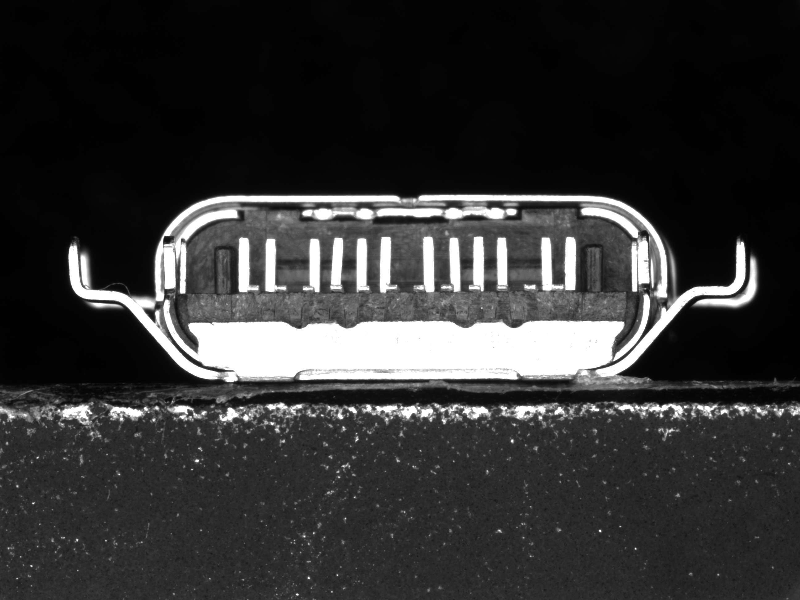
The object of measurement is shown in Figure 20.1: on a 2592×1944 grayscale image, against a dark background, lies the side cross-section of a Micro-USB connector, with a row of contact pins standing inside the bright metal shell. Each pin is a bright vertical metal bar (gray about 240), flanked on both sides by dark background (gray about 70) — sharp contrast, steep boundaries. This is exactly the caliper’s home turf: search horizontally to measure pin width and the spacing between pins. Connector-assembly yield depends heavily on the geometric consistency of the pins; pins that are too wide, too narrow, or misaligned cause abnormal insertion force or poor contact, so pin width and pitch are the critical dimensions of such parts. This chapter takes two adjacent pins (denoted pin A and pin B) as the measurement targets.
20.1 How the Caliper Works
The caliper shares its roots with the search-line machinery of Chapter 14: take a gray profile along the search direction inside the ROI, suppress noise by projection averaging in the perpendicular direction, take the first derivative of the profile, and apply parabolic interpolation at the derivative extremum to obtain the subpixel edge position. If an edge-point extractor outputs “a string of points, left for you to fit”, the caliper differentiates itself in three ways: first, it is natively oriented toward the edge pair — it locates two edges and directly gives the distance between them, i.e. the width; second, when multiple candidate edges appear on the profile, it selects edges by scoring rules such as strength and expected distance, giving it built-in immunity to false edges caused by oil stains and scratches; third, its output is the measurement value itself, with no post-processing required. Its relationship to Chapter 13 can be stated in one sentence: edge detection answers “where in the image are there edges”, while the caliper is the one-dimensional specialization for “we already know roughly where the edge is and need to measure it accurately” — the search range collapses from the full 2D image to a single line, and both speed and accuracy benefit.
The “caliper” takes its name from the mechanical vernier caliper: two jaws grip the workpiece to read out the width. The software caliper is its virtual counterpart — the ROI is the body, and the two edges are the contact points of the jaws. A vernier caliper subdivides the scale with its vernier; a software caliper subdivides the pixel with parabolic interpolation — the idea runs in the same vein.
Let us first lay out the measurement results (Figure 20.2). SciVision’s SDK caliper gives pin A a left edge of x=1003.42, a right edge of x=1036.15, width 32.73 px; pin B a left edge of x=1076.68, a right edge of x=1108.92, width 32.24 px. The center-to-center spacing (pitch) of the two pins is 73.02 px, and the dark gap from pin A’s right edge to pin B’s left edge is 40.53 px. These are direct readings in the pixel domain; if the system is calibrated at \(s\) μm/pixel, the pin pitch is \(73.02\,s\) μm. Note that this SDK’s caliper fit line is always vertical (detailed in Section 20.5), so it measures the horizontal distance; the pins are nearly vertical (the measured tilt via LinePointsLocator is only 0.16°), so the difference between horizontal and perpendicular width appears only in the second decimal place.
This chapter’s SDK output uses the pixel corner coordinate convention (integer pixel boundaries are integers, pixel centers are x.5): pin A’s left edge x=1003.42 lies between columns 1003 and 1004. When comparing subpixel results across libraries, align the coordinate conventions first, or an “error” of 0.5 px will appear out of nowhere.
20.2 Where Subpixel Accuracy Comes From
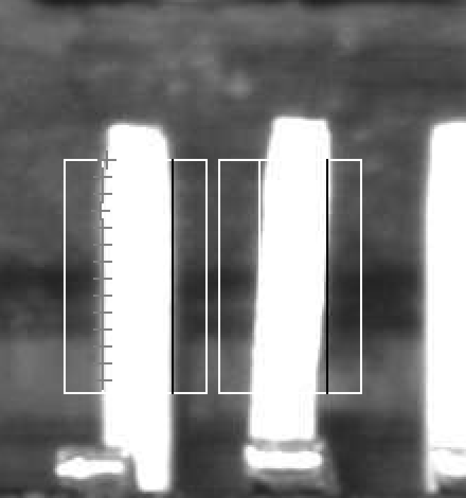
The pixel grid has a spacing of 1; on what basis can we measure an edge to within 0.1 pixel? The answer lies in the physical nature of edges: an edge in a real image is never a mathematical step. The lens point-spread function smears the sharp physical boundary into a gradient, and the photosite further smooths it by integrating the light intensity over its sensitive area (Chapter 3) — by the time it reaches the digital image, the edge is already a gray ramp spanning one to several pixels. Figure 20.3 magnifies pin A’s left edge 8×: between the dark background and the bright pin there is no single cut but a smoothly transitioning gray band, with the “half-gray” pixels plainly visible. The gradient is precisely where the information lives: the true edge position continuously determines the gray value of every pixel in the transition band — move the edge right by 0.1 px and the transition pixels’ gray levels change proportionally. What subpixel localization does is decode the continuous position from the specific values of these few half-gray pixels.

The decoding tool is the parabolic interpolation already used in Chapter 14 (its least-squares roots are in Chapter 2): fit a parabola to the discrete extremum of the profile’s first-derivative magnitude and its neighbors \(g_{-1},g_0,g_{+1}\); the vertex offset \(\delta=\dfrac{g_{-1}-g_{+1}}{2(g_{-1}-2g_0+g_{+1})}\) is the subpixel correction. Figure 20.4 spreads this process out on pin A’s left edge: the gray dots are the raw gray samples of a single row (y=845), jittered by sensor noise; the black polyline is the profile after projection averaging over 111 rows, with a clean ramp outline; the vertical dashed line is the subpixel edge position obtained by interpolating the averaged profile, x=1002.91.
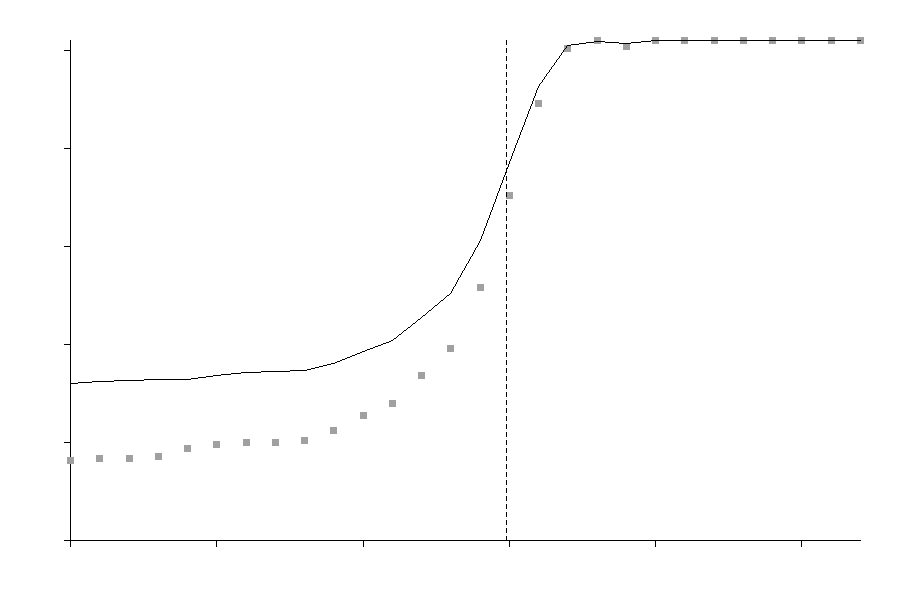
The interpolation formula itself is closed-form; the quality of the accuracy depends on how clean the profile fed to it is. Extracting the subpixel edge row by row on pin A’s left edge, the positions of 111 search rows have a mean of 1002.96 px and a standard deviation of 0.37 px — this 0.37 px contains both sensor noise and the real workpiece geometry (see Section 20.4). The caliper jointly fits these 20 search rows into a single vertical line, and the jitter of the single-point estimate is lowered by \(\sqrt{N}\) averaging, so the final output is far more stable than any single row. This is precisely the subject Section 20.3 will quantify.
20.3 Repeatability: The Lifeline of Measurement
One of the quantities industrial measurement cares about most is: how much do results scatter when the same workpiece is measured repeatedly — repeatability. Precision means “measures steadily” (small variance), accuracy means “measures correctly” (mean close to ground truth); production-line decision logic is built on “the fluctuation of the measurement is far smaller than the tolerance band”, and a system with poor repeatability — even with an unbiased mean — will misjudge good parts as defective and put defective parts into the good pile.
Accurate vs. steady: accuracy bias can be corrected by calibration and standard parts, but random scatter can only be lowered by improving the measurement system itself. The rule of thumb in gauge capability analysis (GR&R): the measurement system’s repeatability (often taken as ±3σ scatter) should not exceed 1/10 of the tolerance band, or measurement error will significantly erode the credibility of the judgment.
A real sample is a single image with no ensemble of noise for a Monte Carlo, so we reproduce repeatability via ROI nudging: translate the caliper ROI up and down along the pin direction by ±8 px (17 positions in total, with a slightly different set of sampled search rows each time), and tabulate the scatter of four measured quantities:
| Quantity | Single measurement (px) | Repeatability σ (px, 17 ROI nudges) |
|---|---|---|
| Pin A width | 32.73 | 0.073 |
| Pin B width | 32.24 | 0.052 |
| Pin pitch (center) | 73.02 | 0.373 |
| Gap width | 40.53 | 0.362 |
The repeatability of both pin widths is in the range 0.05–0.07 px: converted to a typical system at a few μm/pixel, this amounts to sub-0.5 μm single-measurement scatter. The most worthwhile comparison is with the single-row scatter — Section 20.2 measured the per-search-row subpixel edge scatter as 0.37 px, while the caliper jointly fits 20 search rows and the width repeatability drops to 0.073 px, about 1/5 of the single-row scatter; this is exactly the \(\sqrt{N}\) law of Chapter 2: \(0.37/\sqrt{20}\approx 0.083\), on the same order as the measured 0.073. Multi-search-row projection/fitting is repeatability amplification that is nearly free — lengthen the ROI along the edge, add search rows, and the variance of the position estimate falls proportionally, with the ceiling set by how perpendicular the edge is to the search lines.
Why is the σ of pin pitch and gap (0.37, 0.36 px) nearly five times that of a single pin width? Because each is obtained by subtracting the edges of two different pins, two independent ROIs, and the fitting errors of the two ends are no longer as highly correlated as the left and right edges of the same pin, so the scatter is amplified by approximately independent superposition. This is the general rule for composite-quantity measurement: error grows with the number and independence of the participating edges, and measuring pitch is more “delicate” than measuring a single width.
20.4 Precision Is Not Accuracy
The 0.07 px repeatability measured in the previous section is splendid, but it only answers “how steady is the measurement”, not “how correct is it”. This is the most fundamental difference between a real sample and a synthetic scene: a synthetic image carries its own ground truth and lets you compute bias directly; this connector sample has no certified ground-truth pin width whatsoever, so we can only give precision, not accuracy. When reporting the number 32.73 px, we must be honest — its repeatability is 0.07 px, but how far it lies from the true physical width cannot be judged from this image. The only way to complete this link on a production line is to place a standard gauge block whose dimension is certified by a metrology institute, and use it to anchor the pixel reading to physical units and correct the system bias — this is the same thing Chapter 5 stresses with “calibration gives the scale, and calibration expires”.
Real data also reveals a detail invisible on synthetic images: that 0.37 px of per-row scatter is not all noise. The subpixel positions of pin A’s left edge across 111 rows range from 1002.42 to 1004.59, spanning about 2 px — this is not random jitter but a slight taper and curvature of the stamped metal pin’s edge itself, real workpiece geometry. The caliper’s vertical-line fit “presses” this slightly curved edge into a representative straight line, and the 0.37 px mixes two components: sensor noise and part shape. This is an important engineering lesson: do not treat all scatter as noise — sometimes the scatter hides real shape information about the part. If you care whether the pin is bent, you must dig this residual out of the fit and analyze it, rather than smearing it away with ever more averaging.
A synthetic scene can compute bias because the ground truth is written by us; a real sample measures an “unknown part”, and without ground truth there is only precision. This is not a defect but the norm: the vast majority of production-line measurements have no per-part ground truth, relying instead on the combination of standard-part calibration and repeatability monitoring to guarantee credibility.
From this we obtain the chapter’s practical doctrine: when evaluating an algorithm with real parts, report precision and accuracy separately. Repeatability can be measured directly from ROI nudging of a single image, or from repeated captures of the same workpiece; accuracy, however, requires an external standard part. Conflating the two — speaking of “accuracy” with a ground-truth-free sample, or passing off the bias of an idealized synthetic image as real performance — leads to conclusions disconnected from the production-line reality.
20.5 SciVision Implementation
The caliper is provided by SCIMV::SciSvCaliper, but the current state of this module needs honest disclosure. The old interface described in manual section 7.1 is blanked out in the header with an #if 0; what is actually usable is the current Caliper(). It empirically has several behaviors at odds with the documentation: of the polarity parameter, only polarity1=2 can find an edge, and its measured semantics are “from dark to bright along the search direction” — exactly opposite to the header comment; passing 0 or 1 always raises error 122504007; the edge-pair mode (edge2Idx>=1) never outputs a width (widthArr is always 0); the differential caliper mode=1 always fails; and the fitted edge line is always vertical (angle output always 90°). The core function of “the caliper measuring width” is implemented in engineering with a two single-edge-call workaround: inside an ROI containing only a single pin, search once with direction=2 (left to right) and once with direction=3 (right to left) (the dark→bright polarity hits one side of the pin each time), and the difference in x of the two vertical fit lines is the horizontal width:
EdgeDirection dir;
dir.direction1 = direction;  // 2=left-to-right; 3=right-to-left (the two calls hit the two pin sides)
dir.polarity1  = 2;          // empirically the only usable: dark->bright along search (opposite to header)
EdgeFilter filter;
filter.searchLineCount = 20; // 20 search rows inside the ROI
filter.edgeWidth = 3; filter.projectWidth = 1;       // mode=0 already projects over the whole ROI; do not increase
filter.sensitivity = 30; filter.strengthThresh = 30; filter.strengthLimit = 255;
EdgeScoring scoring;
scoring.maxResultNum = 5; scoring.expectDist = 34; scoring.sortMethod = 0;
SCIMV::SciSvCaliper cal;
long rc = cal.Caliper(src, roi, region, /*mode caliper*/0, dir, filter, /*trend*/0,
                      /*pattern specify edge*/0, /*edge1Idx*/1, /*edge2Idx single edge*/0, scoring,
                      &avg, &widthArr, &scoreArr, &mxi, &mni, &pos1, &ang1Arr, &pos2, &ang2Arr);
double edgeX = 0.5 * (pos1[0].x + pos1[1].x);        // fit line is always vertical, both endpoints share x
// pin width = max(e2,e3) - min(e2,e3); pin center = mean of the two edges; pitch = difference of two pin centers
strengthThresh=30 is the first-derivative magnitude threshold; expectDist=34 tells the scorer the expected width scale of the pin; edge1Idx=1, edge2Idx=0 means take only the first edge and do not form an edge pair. The 32.73 px width in Section 20.1 comes from these two calls on pin A. One measured caveat: the pin’s left-edge gradient is strong and stable only within y∈[780,920]; outside this range the contrast at the pin’s tip/root collapses and the caliper raises 122504007; the ROI and search band must fall within the segment where the edge is clear — this is an extra piece of homework that a real sample imposes relative to an idealized synthetic image.
The LinePointsLocator comparison route has triple value: it measures the true width perpendicular to the edge (the SDK caliper can only measure horizontal width, with distortion growing with tilt); it hands back the subpixel point of each search line to the user, making it easy to self-compute per-row scatter and straightness; and it incidentally gives the edge tilt (measured 0.16° for pin A). There is one implementation detail: for near-vertical edges, fit \(x = ay + b\) instead, to avoid FitLine’s defect on vertical point sets (Chapter 14):
SCIMV::SciSvLineLocator loc;
SciPointArray pts;
long rc = loc.LinePointsLocator(src, roi, region, /*strengthThresh*/30,
             /*direction left->right*/2, /*polarity dark->bright*/0, /*edgeWidth*/3,
             /*projectWidth*/1, /*edgeType best*/2, /*searchLineCount*/16,
             /*findPointType first derivative*/1, &pts);
// self-fit x = a*y + b on pts; distance of the two fit lines at the ROI center height / sqrt(1+a^2) is the perpendicular width
It is not uncommon for a commercial SDK’s caliper module to carry such quirks; the countermeasure is the same as in Chapter 14: recompute the key quantities yourself from the raw output, and empirically test the usable range parameter by parameter on the real sample. The complete runnable project is in code/caliper_measurement/.
Industry Case: Glass Width Measurement at 0.01 mm Tolerance
A cover-glass edge-grinding line requires a width tolerance of ±10 μm at an imaging resolution of 5 μm/pixel — the tolerance band converts to ±2 px, and by the 1/10 rule the repeatability must reach 0.2 px. The single-shot caliper repeatability after projection averaging is about 0.07 px (0.35 μm), seemingly with ample margin, yet production data exposed another enemy: the day-night temperature swing of the workshop makes the lens barrel and frame expand and contract, and the measurement mean drifts 0.5 μm over a day — five times the repeatability scatter. Good precision does not mean high accuracy: scatter is “how much a hundred measurements today differ”, while drift is “how much one measurement in the morning and one in the afternoon differ”, and the latter is exactly what the repeatability metric cannot see. The final solution was to place a standard gauge block on the line and re-measure it every two hours, correcting the scale factor in real time — gauge calibration is the bedrock of measurement, the same point as “precision is not accuracy” stressed in Section 20.4 of this chapter.
20.6 Summary
- The caliper is a directed one-dimensional measuring tool: ROI + search direction + polarity frame the problem, and projection, differentiation, and parabolic interpolation give the subpixel edge — it shares roots with the search-line machinery and is the one-dimensional specialization for “we know where the edge is and need to measure it accurately”. On a real Micro-USB connector this chapter measured adjacent pin widths of 32.73 / 32.24 px, a center pitch of 73.02 px, and a gap of 40.53 px.
- Subpixel information lives in the gradient: the lens PSF and photosite integration smear the edge into a gray ramp whose pixel values continuously encode the edge phase; an 8× magnification of the real pin edge reveals a clear transition band, and parabolic interpolation decodes the subpixel position from it.
- Repeatability is the lifeline of measurement, and multi-search-row averaging is its cheapest amplifier: the per-row subpixel scatter is 0.37 px, and after fitting a straight line over 20 rows the pin width repeatability drops to 0.073 px (≈ 0.37/√20), the mechanism being the \(\sqrt{N}\) law; composite quantities (pitch, gap), by combining the errors of two independent ROIs, amplify the scatter nearly fivefold to 0.37 px.
- Precision is not accuracy: a real sample with no certified ground truth can only give precision (0.07 px), not accuracy; accuracy requires anchoring with an external standard part. The per-row scatter also mixes in the real taper of the stamped pin (about 2 px), which must not be uniformly averaged away as noise.
- Keep an empirical attitude toward the SDK’s caliper module: this version of
Caliper()has polarity semantics opposite to the comment, an edge pair that outputs no width, and an always-vertical fit line, so engineering works around it with two single-edge calls; and one must empirically measure the usable segment where the edge is clear on the sample (the pins are measurable only within y∈[780,920]). TheLinePointsLocatorself-fit route provides perpendicular width and tilt and is a more controllable comparison.
For the accuracy limits of edge localization and the bias-and-variance analysis of various subpixel methods, see the chapters on one-dimensional edge extraction and accuracy evaluation in the work by Steger et al. (Steger, Ulrich, and Wiedemann 2018). One classic origin of subpixel edge localization is Haralick’s step-edge detection via the zero crossing of second directional derivatives under a facet model, which systematically characterizes how edge phase is recovered analytically from a local gray-level polynomial (Haralick 1984). As for the chapter’s recurring theme that “precision is not accuracy” and the evaluation of repeatability and reproducibility (gauge R&R), these belong to gauge capability analysis: AIAG’s Measurement Systems Analysis reference manual lays out the standard procedures for assessing repeatability, reproducibility, bias, and linearity, and is the authoritative bridge from this chapter’s scatter numbers to production-line judgment specifications (Automotive Industry Action Group 2010).