3 Cameras and Lenses
However ingenious the algorithms in a machine vision system may be, they only ever process the image the camera hands over. At the very top of the algorithmic chain sits the optics: the moment light passes through the lens and lands on the sensor, the upper bound on image quality is already fixed — insufficient contrast, smeared detail, motion blur, perspective distortion: none of these defects can be truly repaired by any downstream algorithm. Spending money and thought on choosing the right camera and lens is usually a far better deal than “enhancing” the image in software after the fact.
This chapter does three things. First, we establish the pinhole imaging model and derive the selection calculations that link focal length, working distance, and field of view. Next, we discuss the key engineering concepts on the sensor and lens side — pixels, shutters, depth of field, and telecentricity. Finally, we answer a question that gets asked on the production line every single day: can “sharp” be turned into a number? We will present two families of focus measures, compare their merits with a set of real experiments, and explain how autofocus “climbs the hill” along the resulting curve.
3.1 The Pinhole Model and Imaging Geometry
The simplest and most useful camera model is the pinhole model: all rays pass through an ideal small aperture and form an inverted image on an image plane at distance \(f\) behind it. Let a point in space have coordinates \((X, Y, Z)\) in the camera frame (\(Z\) being the distance along the optical axis); its image-point coordinates are
\[ x = f\,\frac{X}{Z}, \qquad y = f\,\frac{Y}{Z}. \]
This is perspective projection, and its heart is that division by \(Z\): an object of the same size images smaller the farther it is from the camera (the larger \(Z\) is) — the everyday experience of “near things look big, far things look small” compressed into a single division. The parameter \(f\) is the focal length, the scaling knob of the imaging geometry: the longer \(f\), the larger the image of a given object and the narrower the field of view.
Real lenses also exhibit distortion: straight lines bend into arcs on the image plane, increasingly so toward the edge of the field. Chapter 5 will add distortion terms and the intrinsic matrix on top of the pinhole model to obtain a complete model fit for precision measurement; in this chapter the ideal pinhole is enough to build selection intuition.
The quantities used most often in lens selection are connected through this model. Let the working distance (WD) be the distance from the lens to the object, the field of view (FOV) be the width of the object plane that the image just covers, and \(h\) be the sensor width; then the magnification is
\[ m = \frac{h}{\mathrm{FOV}}, \qquad f = \frac{m\cdot \mathrm{WD}}{1+m}. \]
The second equation follows from the thin-lens formula; when \(\mathrm{WD} \gg f\) it degenerates into the more familiar rough form \(f \approx m\cdot\mathrm{WD}\).
Let us work a concrete example. An inspection station uses a 1/1.8″ sensor with 2.4 μm pixels and a resolution of 3072×2048, giving a sensor width of \(h = 3072 \times 2.4\ \mu\text{m} \approx 7.4\) mm; the mechanics fix the working distance at 300 mm, and a field of view 50 mm wide must be covered. Thus \(m = 7.4/50 \approx 0.148\), and substituting gives \(f \approx 0.148 \times 300 / 1.148 \approx 38.7\) mm. No off-the-shelf fixed-focal-length lens comes in a 38.7 mm step, so we round down to the nearest 35 mm: the actual magnification becomes \(m' = f/(\mathrm{WD}-f) = 35/265 \approx 0.132\), and the actual field of view about \(7.4/0.132 \approx 56\) mm — slightly wider than required, which leaves margin for mounting and alignment; choosing 50 mm instead would shrink the field to about 37 mm, simply not enough. Finally, check the spatial resolution: 56 mm spread over 3072 pixels gives about 18 μm per pixel. Whether that number suffices depends on the rule of thumb in the next section.
3.2 Sensors and Pixels
A pixel is a photosensitive cell on the sensor — in essence a “well” that collects photogenerated electrons. The maximum number of electrons one well can hold is called the full well capacity; the ratio of full well capacity to readout noise determines the dynamic range — the span between the brightest and darkest values that can be distinguished within a single image. Chapter 1 discussed bit depth: whether 8-bit or 12-bit quantization is meaningful comes down, in the end, to whether the sensor’s dynamic range can support that many gray levels — otherwise the extra bits merely quantize the noise more finely.
This leads to a pair of frequently overlooked trade-offs: for a sensor of the same size, higher resolution means smaller pixels. As pixels shrink, the full well capacity scales down with the photosensitive area, the signal-to-noise ratio and dynamic range degrade in step, and brighter illumination or longer exposure is needed to feed them. “The higher the resolution, the better” is the most common fallacy in camera selection — resolution should be calculated from the requirement, not maxed out to the budget.
How is the requirement calculated? Rule of thumb: the smallest defect or smallest feature must cover at least 2 pixels — exactly the engineering version of the sampling theorem from Chapter 1 (in practice, 3–4 pixels are often used for margin). The example in the previous section gave 18 μm per pixel, meaning the smallest reliably detectable defect is about 36–70 μm; if the process requires detecting 20 μm defects, the field of view must be shrunk or a higher-resolution solution adopted.
Another question that must be settled before the purchase order goes out is the shutter type. A global shutter starts and ends the exposure of all pixels at the same instant, yielding a true “single moment in time”; a rolling shutter exposes row by row, so the top and bottom of one frame are separated by a full readout period. For a stationary workpiece the two are indistinguishable, but the moment the workpiece or the camera moves, a rolling shutter turns rectangles into parallelograms and circles into eggs — a geometric distortion caused by the row-by-row time offset that no calibration can remove after the fact. The conclusion is hard: workpieces in motion (fly-by capture on a conveyor, snapshots on a moving stage) require a global shutter. Rolling-shutter sensors are cheaper and often lower in noise, and are suitable only for stationary-capture scenarios.
3.3 Depth of Field and Telecentric Lenses
In the pinhole model everything is in focus everywhere; a real lens has only one plane of focus. When an object departs from that plane, each object point spreads into a small blur spot on the image plane; as long as the spot diameter does not exceed the circle of confusion \(c\) (in engineering practice typically 1–2 pixels), both humans and algorithms still judge it “sharp”. The front-to-back range over which sharpness is maintained is called the depth of field (DOF), approximately
\[ \mathrm{DOF} \;\approx\; \frac{2\,c\,N\,(m+1)}{m^{2}}, \]
where \(N\) is the f-number. Read this formula qualitatively: stopping down the aperture (increasing \(N\)) increases the depth of field — at the cost of light throughput falling as \(N^2\), and beyond a certain point diffraction makes the whole field soft instead; the magnification \(m\) sits in the denominator squared, so the depth of field collapses extremely fast at high magnification — microscopic observation has a sharp layer as thin as paper. When the depth of field is insufficient, first consider stopping down and adding illumination, then reducing the magnification, and only as a last resort flattening the workpiece mechanically.
Ordinary lenses also have an inherent problem unrelated to focus: perspective error. From \(x = fX/Z\), the magnification varies with \(Z\): \(\Delta m / m \approx \Delta Z\,/\,Z\). Returning to the example of the previous section: with a working distance of 300 mm, a workpiece surface undulation or fixture repeatability of ±1 mm changes the magnification by ±0.33%, introducing a reading drift of ±0.17 mm over a 50 mm measured dimension — catastrophic for dimensional measurement with tolerances of a few micrometers. And this is not a focus problem; stopping down will not save you.
The telecentric lens exists precisely for this: the aperture stop is placed at the image-side focal plane, so that all object-side chief rays are parallel to the optical axis. Within the telecentric range, therefore, the magnification does not vary with object distance — the workpiece can wobble, be thicker, sit tilted, and the image size does not budge; perspective error is eliminated by the optical structure itself. The price is size, weight, and cost. When is a telecentric lens mandatory? High-precision dimensional measurement (tolerances down at the micrometer level), measured objects with thickness or steps (an ordinary lens images the upper and lower surfaces at different magnifications), and situations where the \(Z\) position cannot be tightly controlled.
The hard constraint of telecentric lenses: because the chief rays are parallel to the optical axis, the front group’s aperture must be no smaller than the measured object — measuring a 50 mm workpiece requires a telecentric lens with an aperture exceeding 50 mm. This is the fundamental reason telecentric lenses are large and expensive, and why they are normally used only at measurement stations, not for large-field locating.
3.4 Quantitative Evaluation of Sharpness
In the lab, “is the image sharp?” is judged by eye; on the production line, it must be judged by a number: autofocus needs an objective function to search over; equipment alignment and acceptance need a metric that can be written into the process document; comparing old and new lenses, or lenses from different batches, needs one common yardstick. A function that maps an image to a single scalar for this purpose is called a focus measure; a good one takes a unique peak at best focus and decreases monotonically with defocus.
The most direct idea comes from observation: when an image blurs, what is lost is high-frequency detail — edges become gentle. The gradient-energy method (the Tenengrad idea) directly measures how “steep” the edges are:
\[ S_{\mathrm{grad}} = \frac{1}{NM}\sum_{n,m} \Big( G_x[n,m]^{2} + G_y[n,m]^{2} \Big), \]
where \(G_x\) and \(G_y\) are the horizontal and vertical gradients (e.g., Sobel operator responses). The sharper the image, the larger the gradient magnitudes and the higher the score. The other family is the gray-level variance method, which measures how far the whole image’s gray values depart from their mean:
\[ S_{\mathrm{var}} = \frac{1}{NM}\sum_{n,m} \big( g[n,m] - \bar g \big)^{2}, \qquad \bar g = \frac{1}{NM}\sum_{n,m} g[n,m]. \]
Blur is a form of averaging: it squeezes gray values toward the mean, and the variance drops accordingly — it is the fastest to compute, but what it measures is global contrast, not detail. Which of the two is better? Let the experiments speak.
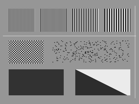
We synthesize a 480×360 test scene (Figure 3.1): the top row holds four groups of vertical stripes with periods of 2, 4, 6, and 8 px, the equivalent of a simple resolution chart; the middle row holds a 4 px checkerboard and a block of random speckle simulating text-like texture; the bottom row holds a dark rectangle providing step edges and a diagonal black-and-white edge; in addition, two bright lines 1 px wide run across the frame. From the finest 1 px structures to the coarsest large light-and-dark blocks, every spatial scale is represented.
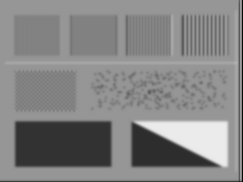
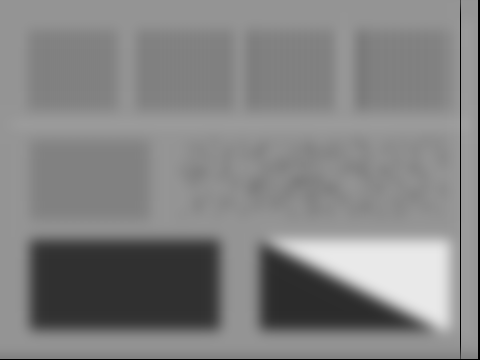
We then simulate progressive defocus with Gaussian blur (a real defocus spot is approximately a uniform disk of confusion; the Gaussian is its smooth first-order approximation — see Chapter 6 for the filter itself), with \(\sigma\) taking the seven levels 0, 0.8, 1.6, 2.4, 3.2, 4.8, 6.4, and the kernel size chosen as the odd number near \(K \approx 6\sigma\). Figure 3.2 shows two of the levels: at \(\sigma=2.4\), the fine stripe groups with periods of 2 px and 4 px have completely melted into uniform gray blocks — that detail is gone for good — while the coarse stripes, the rectangle, and the diagonal edge survive; at \(\sigma=6.4\), all stripes and the checkerboard are wiped flat, and only large patches of light and dark remain.
For each blur level we compute both scores and normalize them to 1 at \(\sigma=0\); the results are given in Table 3.1 and Figure 3.3.
| Blur \(\sigma\) | Gradient (normalized) | Variance (normalized) |
|---|---|---|
| 0.0 | 1.0000 | 1.0000 |
| 0.8 | 0.7330 | 0.6693 |
| 1.6 | 0.3441 | 0.5125 |
| 2.4 | 0.1850 | 0.4716 |
| 3.2 | 0.1356 | 0.4552 |
| 4.8 | 0.1145 | 0.4302 |
| 6.4 | 0.1053 | 0.4068 |
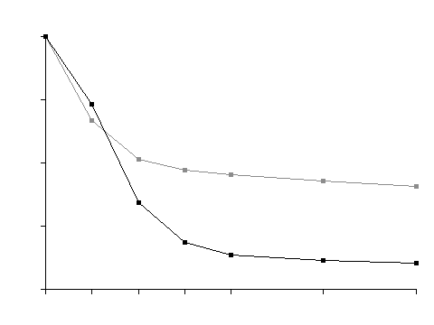
Both curves decrease strictly monotonically — either is “usable” as an autofocus objective — but the difference in quality is dramatic. The gradient method discriminates far better than the variance method: from \(\sigma=1.6\) to 6.4, the gradient score drops from 0.344 all the way to 0.105 (a span of more than 3×), while the variance score eases only from 0.513 to 0.407, hitting a plateau early. The reason goes back to the nature of the two formulas: what blur erases is high-frequency detail, while the large light-and-dark structures — the dark rectangle, the diagonal edge — retain their global contrast at any blur level. The variance method looks only at contrast, so even when the image has blurred into nothing but color patches it still awards forty percent of the score; the gradient method watches the steepness of edges and reacts far more sensitively to the loss of detail. A focus measure with poor discrimination means a focus curve with a flat peak region and a nearly flat far-defocus region — the search algorithm can neither judge direction nor decide convergence.
Given a monotonic focus curve, autofocus is hill climbing on that curve: move the focus motor or the \(Z\) axis, capture and score an image at each position, keep going in the direction of rising score, and stop once past the peak. The practical search strategy is coarse-to-fine in two stages: first sweep the whole travel with a large step to bracket the peak within an interval (also steering clear of noise artifacts on the far-defocus plateau); then scan that interval with a small step and fit a parabola to the few samples near the top, interpolating the best focus position to within a fraction of the step. The better the focus measure’s discrimination, the more reliable the direction decisions in the coarse sweep, and the narrower the fine-scan interval can be drawn.
An engineering detail: the Gaussian filter of the SDK used in this experiment does not fix its internal floating-point summation order, so on a rerun the 3rd significant digit of the scores jitters slightly (at \(\sigma=0\) no filtering is applied and the scores match digit for digit), but the monotonicity and discrimination conclusions are stable. With evaluation-type metrics, engineering judgment should rest on trends and orders of magnitude, not on the last digit.
3.5 SciVision Implementation
Focus measures are provided in the SciVision SDK by the SCIMV::SciSvFocus class, whose core interface is GetFocusScore:
SCIMV::SciSvFocus focus;
SciROI roi;
SciPoint tl(0, 0), br(W - 1, H - 1);   // GenRect1 takes non-const references, so named variables are required
roi.GenRect1(tl, br);

double score;
long rc = focus.GetFocusScore(frame, roi, SCI_GRADIENT, &score);
if (rc) { /* non-zero is an error code and must be checked */ }
The four parameters are, in order: srcImage, the image to be evaluated; ROI, which restricts the evaluation region and supports three types — axis-aligned rectangle, rotated rectangle, and undefined, where the undefined type means the whole image is processed (on the production line the ROI is usually framed around the feature under test to keep the background from contaminating the score); method, which selects the evaluation algorithm, see the table below; and score, which returns the result. The score is a relative quantity: it is only meaningful to compare scores obtained on the same scene, the same ROI, and the same method.
GetFocusScore
| Enum value | Method | Characteristics per the manual |
|---|---|---|
SCI_VARIANCE (0) |
Variance method | Sensitive to noise, shortest runtime |
SCI_EVA_IMPROVE |
Point-sharpness method | Fairly sensitive to noise and missing detail, longest runtime |
SCI_IMAGE_DIFFERENCE |
Difference method | Fairly sensitive to noise and missing detail, longer runtime |
SCI_GRADIENT (3) |
Gradient method | Less affected by noise and missing detail, longer runtime |
This chapter’s experiments use the SCI_GRADIENT and SCI_VARIANCE settings, corresponding to the two formulas of Section 3.4. The SDK also provides ScoreStatistics and CurveFitting, for finding the highest point in a score sequence and for optimally fitting the score curve respectively — ready-made building blocks for the autofocus “coarse sweep — fine sweep — peak fitting” procedure. The complete project that generates all of this chapter’s images and score tables is located at code/cameras_and_lenses/; readers can modify the scene structure and blur parameters to reproduce the results themselves.
Industry Case: Lens Assembly Acceptance on the Line
After a module maker’s inspection equipment was duplicated onto a second production line, the false-detection rate was noticeably higher. The investigation traced it to assembly technicians focusing by eye: “looks about sharp” is simply not reproducible across different people and different monitors. The remedy was to write the focus score into the alignment/assembly process: after each unit is assembled, it photographs a uniform standard target and is scored with GetFocusScore (gradient method); only units reaching at least 95% of the benchmark unit’s score are released. Two pitfalls are worth recording. First, the focus score is highly sensitive to the imaged content — swap in a different target sheet and the scores lose all comparability, so acceptance must use a standard target of the same model in the same pose. Second, the last digits of the score exhibit floating-point jitter, which is entirely absorbed once the threshold carries a 5% margin — an acceptance criterion should never have depended on the third decimal place anyway. Once the procedure was locked in, the new line passed alignment on the first attempt, and aging units with focus drift were automatically caught by periodic re-inspection.
3.6 Summary
- The upper bound on image quality is fixed on the optics side, and no downstream algorithm can recover what is lost; selection calculations start from the pinhole model — \(m = h/\mathrm{FOV}\), \(f = m\cdot\mathrm{WD}/(1+m)\) — and then check the object-plane size each pixel covers.
- Calculate resolution from the requirement; do not buy it by budget: the smallest feature must cover at least 2 pixels (3–4 with margin); on a sensor of the same size, smaller pixels mean worse full well capacity and dynamic range. Moving workpieces require a global shutter.
- Depth of field \(\propto cN(m+1)/m^2\): trade aperture for depth of field; at high magnification the depth of field collapses sharply. An ordinary lens’s magnification varies with object distance (\(\Delta m/m \approx \Delta Z/Z\)), so high-precision dimensional measurement requires a telecentric lens, whose aperture must be no smaller than the measured object.
- Sharpness can and should be quantified: the gradient-energy method measures high-frequency detail and discriminates far better than the gray-level variance method, which sees only global contrast (a tail-end gap of 0.105 versus 0.407 in this chapter’s experiment); autofocus is a coarse-to-fine hill-climbing search on the focus curve.
- Focus scores are relative quantities: comparable only on the same scene, the same ROI, and the same method; when used as an acceptance criterion, fix a standard target and leave threshold margin for floating-point jitter.
For systematic selection of cameras, lenses, and illumination, and a more complete optical analysis of telecentric imaging, see the book by Steger et al. (Steger, Ulrich, and Wiedemann 2018); for the geometric derivations of the pinhole model, thin-lens imaging, and perspective projection, see Szeliski’s textbook (Szeliski 2022). This chapter compared only two focus measures — the gradient-energy and gray-level variance methods; to select among a much larger operator set, Pertuz et al. (Pertuz, Puig, and Garcia 2013) evaluate more than thirty focus-measure operators within a unified framework for robustness to noise, window size, and image content, a practical reference when picking a focus measure for autofocus or shape-from-focus.