10 Geometric Transforms

Workpieces on a production line never show up in the field of view at the same position and the same angle every time: vibratory bowl feeders deliver parts with scattered poses, pallet positioning has mechanical play, and pick-and-place nozzles add rotational offsets of their own. Fixturing (position correction) has to “straighten” the image before measuring, multi-camera stitching has to align several images into one coordinate system, and template matching often requires rescaling the image to a suitable resolution first — the common core of all these tasks is the geometric transformation: moving an image from one coordinate system to another. It looks like nothing more than “shift it a little, turn it a little,” yet hidden inside are two questions that must be answered separately: how do the coordinates map — that is the matrix’s job; where do the new pixel values come from — that is interpolation’s job. Get either one wrong and the image develops holes, jagged edges, or a creeping blur — and blur is the sworn enemy of measurement accuracy.

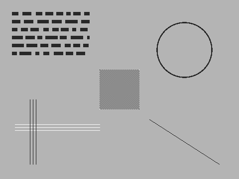
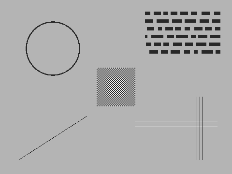
The experiments in this chapter use the 480×360 synthetic scene shown in Figure 10.1. Every structure in it is deliberately designed to give geometric transforms a hard time: the text-like block in the upper left tests detail preservation, three 1 px bright horizontal lines and three 1 px dark vertical lines test thin-line survival, a 1 px diagonal line tests oblique structure, the central 80×80 checkerboard with 2 px squares is the high-frequency pattern most sensitive to resampling, and the ring in the upper right is for observing edge smoothness.

Figure 10.1: The test scene for this chapter (480×360): a text-like block, triplets of 1 px thin lines (horizontal/vertical), a 1 px diagonal line, a central checkerboard with 2 px squares, and a ring — all fine structures sensitive to interpolation and resampling.

10.1 Transformation Matrices

A two-dimensional point \((x, y)\) is written in homogeneous coordinates as \((x, y, 1)^\mathsf{T}\) (see the linear algebra section of Chapter 2), whereupon translation, rotation, and scaling all unify into a single \(3\times 3\) matrix multiplication:

\[ T(t_x,t_y)=\begin{bmatrix}1&0&t_x\\0&1&t_y\\0&0&1\end{bmatrix},\qquad R(\theta)=\begin{bmatrix}\cos\theta&-\sin\theta&0\\ \sin\theta&\cos\theta&0\\0&0&1\end{bmatrix},\qquad S(s_x,s_y)=\begin{bmatrix}s_x&0&0\\0&s_y&0\\0&0&1\end{bmatrix}. \]

Composing them arbitrarily (multiplying the matrices) yields the most general form, the affine transformation:

\[ A=\begin{bmatrix}a_{11}&a_{12}&t_x\\ a_{21}&a_{22}&t_y\\ 0&0&1\end{bmatrix}, \]

with 6 degrees of freedom in total; it keeps straight lines straight and parallel lines parallel. The entire action chain of fixturing — “first translate the workpiece to the center, then rotate it upright about the center” — is mathematically nothing but several such matrices multiplied into one.

Here the real payoff of homogeneous coordinates shows itself: translation is inherently an addition, but after lifting one dimension it becomes a multiplication too, so a transformation chain of any length can be pre-multiplied into a single matrix. This seemingly trivial algebraic fact will turn into an engineering discipline that governs image quality in Section 10.3.

With the matrix in hand, the next question is how to use it to generate the new image. The intuitive approach is forward mapping: walk over every pixel of the source image, compute where it lands in the destination image, and carry the gray value over. This approach has a fatal flaw — the landing coordinates are generally not integers, and after rounding, some destination pixels are fought over by multiple source pixels while others are never hit even once, leaving swaths of holes, especially conspicuous under rotation and magnification. The correct approach is exactly the reverse, called inverse mapping: walk over every pixel \(\mathbf p'\) of the destination image and use the inverse matrix to find its source coordinates in the original image

\[ \mathbf p = A^{-1}\,\mathbf p', \]

then go to the source image and “fetch” the gray value at this (generally non-integer) position. Every output pixel is assigned exactly once, and holes vanish at the root. The handwritten rotation in this chapter’s companion code is implemented on exactly this principle. As for “how to fetch a gray value at a non-integer position” — that is precisely the topic of the next section.

10.2 Interpolation

The source coordinates \((s_x, s_y)\) computed by inverse mapping fall between the pixel grid points, so a gray value must be estimated from the neighboring pixels — this is interpolation. The two basic methods were already introduced in Chapter 2; here we only recap. Nearest-neighbor interpolation simply takes the nearest pixel after rounding; it produces no new gray values, at the cost of a position quantization error on the order of 0.5 px. Bilinear interpolation takes a distance-weighted average of the surrounding 4 pixels: writing \(x_0=\lfloor s_x\rfloor\), \(y_0=\lfloor s_y\rfloor\) and the fractional parts \(a=s_x-x_0\), \(b=s_y-y_0\), then

\[ f(s_x,s_y)\approx(1-a)(1-b)\,f_{00}+a(1-b)\,f_{10}+(1-a)\,b\,f_{01}+ab\,f_{11}, \]

where \(f_{00},f_{10},f_{01},f_{11}\) are the top-left, top-right, bottom-left, and bottom-right neighbors. It outputs continuously transitioning gray values — in essence a slight local smoothing.

How much do they differ? We rotate the test scene by 17° with handwritten inverse-mapping implementations of nearest neighbor and bilinear (the two code paths are identical except for the sampling step); the results are in Figure 10.2. We then crop the central checkerboard region and magnify it 4 times for pixel-by-pixel viewing in Figure 10.3.

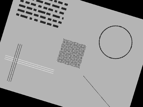
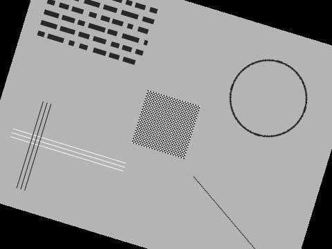
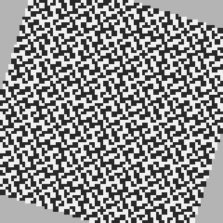
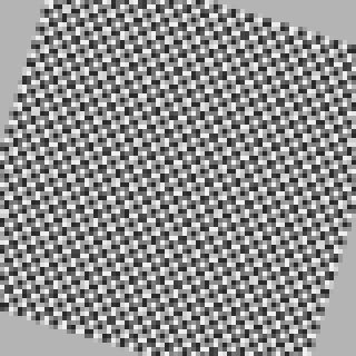
The difference is plain to see: the nearest-neighbor rotation is covered in jaggies, and because each output pixel “jumps” to its nearest source pixel, the black and white squares of the 2 px checkerboard are scrambled into irregular fragments; the bilinear result has smooth edges and tidy geometry, at the price of introducing intermediate gray values that did not exist in the original, so fine structures go slightly soft.

Rule for choosing the interpolation method: measurement tasks (edge localization, calipers, registration) use bilinear or higher-order interpolation, to keep nearest neighbor’s position quantization from harming subpixel accuracy; binary masks and label images must use nearest neighbor — bilinear would interpolate a flood of intermediate gray values between 0 and 255, and the mask would no longer be a mask.

10.3 The Cost of Resampling

The “slight smoothing” side effect of bilinear interpolation is almost invisible after a single pass, but every geometric transform resamples the image once, and the smoothing stacks up one layer at a time. To quantify this cost, we run an experiment that can “return to the starting point”: rotate the test scene by 10° with bilinear interpolation, then by another 10°… 36 times in all, for a total angle of exactly 360° — the image should come back to its original place without a single discrepancy. The result is in Figure 10.4.

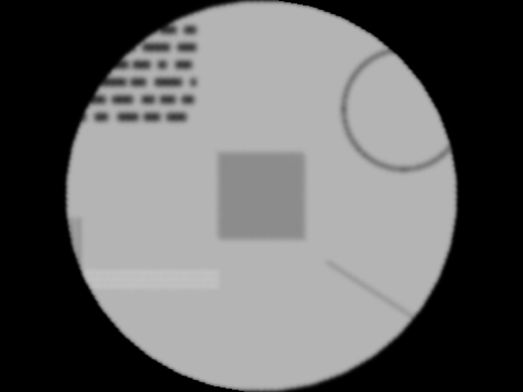
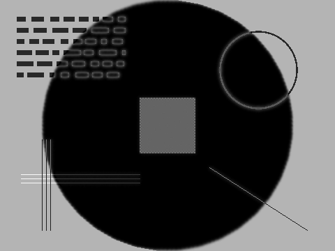
The position did indeed come back, but the image is unrecognizable: the 2 px checkerboard has blurred completely into a uniform gray, the 1 px thin lines are reduced to faint traces, and every corner of the text block has been rounded off. Quantitatively, within the central disk of radius 170 px (avoiding the corner-clipped region), the mean absolute difference (MAD) between the 36-rotation image and the original is as high as 10.78 gray levels; as a control, a single-step rotation by 360° (mathematically the identity transform) has a MAD of 0.0000 — not a single byte inside the disk changed. Chaining the SDK’s rotation interface 36 times gives 10.77, matching the handwritten implementation — proof that this is not a defect of any particular implementation but a property of resampling itself: every resampling is an irreversible loss of information.

The full-frame MAD is 78.57, far larger than the in-disk 10.78 — it is dominated by corner clipping: with isChangeSize=false the frame stays fixed, each rotation swings the corners out of frame and fills them with the fill color, and after 36 rotations only an inscribed disk survives at the center. When computing error statistics, be sure to exclude this region — otherwise you are measuring clipping, not interpolation.

From this follows the most important engineering discipline of the chapter: compose transformation matrices freely in the math; never execute them step by step on the image. When you need “translate first, then rotate, then scale,” multiply the three matrices into one in code and perform exactly one inverse-mapping resampling — the result is mathematically equivalent to doing it in three steps, but in image quality the two are worlds apart.

Corner clipping is itself a semantic issue to watch: the rotation interface’s isChangeSize parameter decides whether the output frame is enlarged to contain the full bounding rectangle of the rotated image. With false, the frame matches the original, corner content is cut off, and the vacated regions are filled with the specified color; with true, the content is preserved losslessly but the frame grows and every downstream ROI coordinate is invalidated. Fixturing-style applications usually choose false and make sure the measured region lies inside the safe disk.

10.4 Scaling and Aliasing

Scaling is also a geometric transform, but downsampling has a trap that rotation does not. Shrinking an image by a factor of 4 means the sampling rate drops to 1/4; by the sampling theorem discussed in Chapter 1, structures in the original with a period shorter than 8 px simply cannot be represented at the new sampling rate, and if left untreated they come back disguised as aliasing (see Chapter 11 for the frequency-domain explanation). The correct procedure is prefilter, then decimate: first filter out the components above the new Nyquist frequency, then reduce the resolution.

We compare using the SDK’s Sampling interface: NEAREST mode amounts to taking 1 sample out of every 4 directly (no prefiltering), while AREA mode amounts to averaging each 4×4 source region (box prefiltering) before decimating. The results are in Figure 10.5 (for easier viewing, both downscaled images have been magnified back to the original size with nearest neighbor, which introduces no new information).

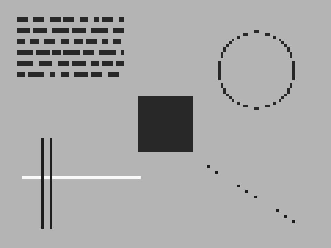
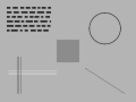
The direct-decimation result is shocking: the 2 px checkerboard aliases into a solid dark patch — the samples happen to land on the dark squares every time, and the high-frequency pattern masquerades as a low-frequency structure that never existed; of three identical 1 px bright lines only one “survives,” the other two happening to be skipped by the sampling, their fate determined entirely by their position relative to the sampling grid; the ring and the diagonal break into dashes. The prefiltered result keeps every structure: the checkerboard averages to mid-gray (its only honest representation at the lower resolution), and all three thin lines remain visible, merely fainter because their energy has been spread thin. Downsampling must be prefiltered — missed detections of thin line-like defects very often trace back to one “convenient” direct decimation in a thumbnail pipeline.

Sampling offers 6 interpolation modes; the applicable scenarios are tabulated below.

Mode	Meaning	Applicable scenarios
`LINEAR`	Bilinear	General-purpose default: magnification, mild shrinking
`NEAREST`	Nearest neighbor (direct decimation/copy)	Binary masks and label images; aliases when downsampling
`CUBIC`	Bicubic (4×4 neighborhood)	High-quality magnification, edges sharper than bilinear
`AREA`	Area averaging (built-in box prefiltering)	First choice for downsampling
`LANCZOS4`	8×8 Lanczos-windowed sinc	Highest-quality scaling; may ring near strong edges
`WEIGHT`	SDK custom weighted mode	Behaves close to LINEAR; verify by measurement before use

10.5 Mirroring, Cropping, and Stitching

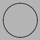
A few common “integer-level” geometric operations remain; they involve no interpolation, move pixels byte by byte, and lose no information. Mirroring performs horizontal (left-right) and vertical (top-bottom) flips, commonly used to unify the orientation of images from symmetric stations or images reflected by prisms. Cropping extracts an ROI region into a standalone small image, reducing the data volume for subsequent processing. Here is an engineering fact that must be remembered: the bottom-right corner of SciVision’s GenRect1 rectangular ROI is an exclusive endpoint — passing (305,35)–(434,164) yields a 129×129 output, not 130×130 (Figure 10.6). Writing code on the “both ends inclusive” intuition will systematically drop the last row and column. Stitching composes multi-camera or multi-view images into a large image; Section 5.12 of the SDK user manual provides the corresponding interfaces, which this book does not expand on.

10.6 SciVision Implementation

Rotation and translation are provided by SciSvRotationShift, a single interface that does both jobs at once:

SCIMV::SciSvRotationShift rot;
SciColor fill(0, 0, 0);          // fill color for regions rotated out of frame
SciImage dst;
// rotate 17° about the image center, frame unchanged, translation (0,0)
long rc = rot.RotateShiftImage(src, fill, 17.0f,
                               /*isChangeSize=*/false, 0, 0, &dst);

The parameters are, in order: input image, fill color, rotation angle (degrees), isChangeSize (whether to enlarge the frame to contain the full rotated result; see Section 10.3 for the semantics), x/y translation amounts, and the output image. Two measured facts must be known. First, this interface exposes no interpolation-method parameter. We compared the SDK’s rotation result for +17° against the handwritten implementation’s −17° rotation (the SDK’s positive-angle direction is opposite to the textbook convention — see the second fact; the negated angle is the same geometric transform; statistics taken within the central disk of radius 170): the MAD against handwritten bilinear at −17° is 1.05, and against handwritten nearest neighbor at −17° is 3.90 — evidence that its interior is a bilinear-class smooth interpolation, safe to use in measurement pipelines; and for the same reason, this chapter’s nearest-neighbor/bilinear comparison experiments were done with the handwritten inverse mapping (the SDK exposes no nearest-neighbor mode). Second, the rotation direction for positive angles is opposite to the common counterclockwise convention: the same +17° given to the SDK and to code implemented per the textbook convention rotates in opposite directions. When porting code from OpenCV or similar libraries, always verify the direction with an asymmetric image first, then settle the sign of the angle.

Scaling, mirroring, and cropping are invoked as follows:

SCIMV::SciSvSampling smp;
SciImage down;
smp.Sampling(src, src.Width() / 4, src.Height() / 4,
             SCI_SV_RESAMPLE_AREA, &down);   // use AREA for downsampling (built-in prefiltering)

SCIMV::SciSvMirror mir;
SciImage flipped;
mir.Mirror(src, SCI_MIRROR_HOR, &flipped);   // horizontal mirror (left-right flip)

SCIMV::SciSvImageCropping cropper;
SciROI roi;
SciPoint tl(305, 35), br(434, 164);          // bottom-right corner is an exclusive endpoint
roi.GenRect1(tl, br);
SciImage patch;
cropper.ImageCrop(src, roi, 0, 0, &patch);   // output is 129×129

The parameters of Sampling are the input image, target width, target height, interpolation mode (see the table in Section 10.4 for choosing among the 6 modes), and the output image; the second parameter of Mirror is the mirror type; the third and fourth parameters of ImageCrop are the cropping type and the out-of-bounds fill gray value. All return codes should be checked. The complete project that generates all of this chapter’s experimental images is located at code/geometric_transforms/.

Industry Case: The Invisible Blur in a Fixturing Chain

A placement-inspection project ran the pipeline “template localization → rotation correction → caliper measurement.” During debugging, to make the translation amount and the angle easier to verify separately, an engineer split the correction into two steps: translate once, then rotate once — two resamplings. After the line went into production, the caliper edges’ transition band blurred from about 2 px to 3 px and edge-localization repeatability degraded by roughly thirty percent; checks of the lighting, the lens, and vibration all came up empty. The cause was finally found in the image chain: two bilinear resamplings had stacked two layers of smoothing. After multiplying the translation and rotation matrices into one affine matrix in code and resampling only once, the edge width and repeatability recovered. The deeper lesson goes further: skip the correction entirely when you can — if the downstream tools support pose-aware ROIs, let the ROI rotate with the workpiece (see Chapter 19) and the image never needs to be resampled at all.

10.7 Summary

Geometric transform = matrix + interpolation: homogeneous coordinates unify translation, rotation, scaling, and affine transforms into \(3\times 3\) matrices; generating the image requires inverse mapping — each output pixel samples back into the source image, whereas forward mapping leaves holes.
Choose the interpolation method by task: measurement tasks use bilinear or higher order; binary masks and label images must use nearest neighbor (it introduces no new gray values).
Every resampling is a loss of information: after 36 rotations of 10° back to the starting position the MAD reaches 10.78, while the single-step equivalent transform gives 0.0000. Multiply a transformation chain into one matrix first and resample only once; if a pose-aware ROI will do, don’t touch the image.
Downsampling must be prefiltered: direct decimation aliases high-frequency structures (the checkerboard turns into a solid patch, thin lines vanish at random); use modes with built-in prefiltering such as AREA.
Verify the engineering semantics: RotateShiftImage exposes no interpolation parameter (measured to be bilinear-class) and its positive-angle direction is opposite to the common convention; the bottom-right corner of GenRect1 is an exclusive endpoint — (305,35)–(434,164) crops a 129×129 region.

The standard treatment of geometric transforms and resampling interpolation is the textbook by Gonzalez and Woods (Gonzalez and Woods 2018); the widely used cubic convolution interpolation, whose accuracy sits between bilinear and spline interpolation, originates in the paper by Keys (Keys 1981). For a more systematic treatment of geometric transforms and interpolation in measurement systems (including the relationship between projective transforms and subpixel accuracy), see the book by Steger et al. (Steger, Ulrich, and Wiedemann 2018).