21 Geometric Measurement
The lines and circles fitted in Chapter 14 are, in the production line’s eyes, mere intermediates. What gets signed off on an inspection report is never “the line’s direction vector” or “the circle’s parameters”, but numbers like 47.8 px from the camera hole to the top edge, a hole roundness of 0.25 px, whether the panel’s corners are square (a right-angle error of 0.09°) — numbers that can be compared directly against the drawing’s tolerances and decide pass or fail. Getting from primitives to these numbers takes one more stage: geometric measurement — applying exact geometric formulas to the fitted points, lines, and circles to obtain distances, angles, and intersections, and then evaluating parallelism, roundness, and straightness according to the definitions of geometric tolerances. The complete measurement chain is: image → edge points → geometric primitives → geometric quantities → judgment. This chapter cares about two things: how the error at each stage propagates into the final numbers; and how the “band-width” class of geometric tolerance quantities differs fundamentally, in statistical character, from the “position” class of dimensional quantities.
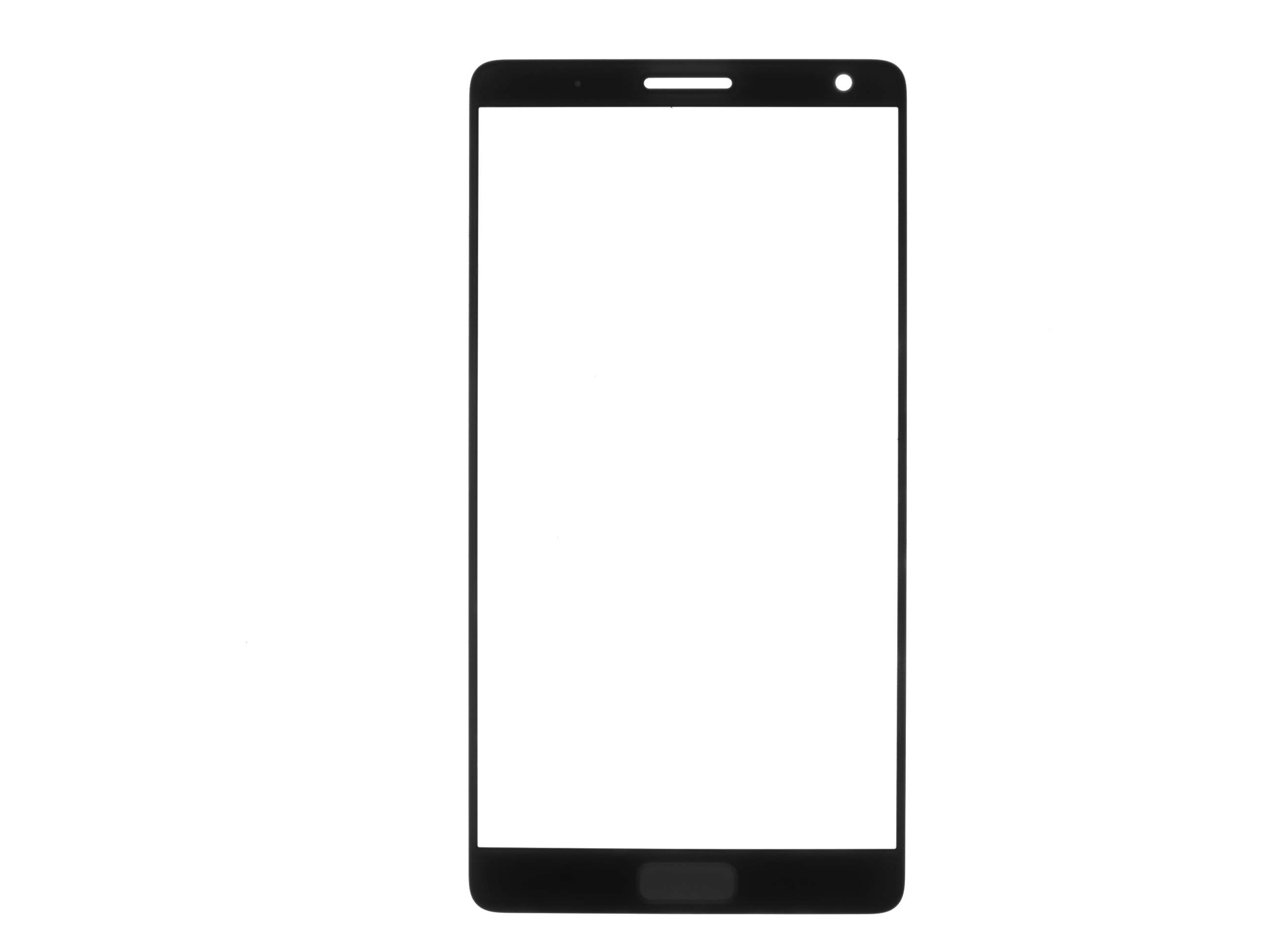
The object of study (Figure 21.1) is a real phone cover glass (a Smart3 “geometric relations” sample image, 2592×1944 single-channel gray): a vertically placed rectangular panel on a white background, whose outer silhouette is a dark bezel, four clean straight edges meeting at the four corners through genuine rounded fillets; the top bezel embeds a circular camera hole and an elongated earpiece slot, and the bottom carries a Home-button bonding pad. This is an extremely common consumer-electronics incoming-inspection part — what the line must measure is exactly the hole position, edge clearances, the panel’s inner and outer dimensions, the squareness of the four corners, and the roundness of the hole. This chapter runs the full geometric-formula kit of Section 21.2 on this real part; unlike a synthetic scene, a real part has no analytic ground truth, so everything below is stated as measured values, with the part’s own geometric self-consistency (the four edges should form an approximate rectangle) serving as a cross-check on measurement correctness.
21.1 The Measurement Chain and Error Propagation
Lay the measurement chain out stage by stage: at the edge-point level, error comes from image noise and the mismatch of the edge model; the primitive level does statistical averaging over many points; the geometric-quantity level consists of deterministic closed-form formulas and introduces no new error of its own — however much the input primitives are off, the output geometric quantities are off by exactly that much; the judgment level compares the geometric quantities against the drawing’s tolerances, and the error budget accumulated over the first three stages directly determines the confidence of the judgment (and how much guard band to leave on the tolerance). So when analyzing the accuracy of a vision gauging system, all the work lies in the error propagation of the first two stages.
The first stage is the edge points. After projection averaging and parabolic interpolation (the machinery of Chapter 14 and Chapter 20), denote the residual noise of a single edge point along the normal direction by \(\sigma_e\). In this example an upper bound on it can be read straight from the fit residuals: the all-point RMSE of the top edge’s 60 edge points about the FitLine least-squares line is only 0.103 px (the left and right long edges are 0.137 and 0.211 px). This RMSE contains both sensor noise and the slight real form undulation of the straight edge itself, so \(\sigma_e \lesssim 0.1\) px is a conservative upper bound — after passing through the whole pipeline, pixel-scale imaging noise has been squeezed below a tenth of a pixel.
The second stage is fitting. Fit a line through \(N\) independent points, and the parameter error shrinks as \(1/\sqrt N\); for the direction there is a second lever as well — the span \(L\) of the point set. For \(N\) points spread uniformly over a span \(L\), the standard deviation of the least-squares line’s direction is approximately
\[ \sigma_\theta \approx \frac{\sigma_e}{L}\sqrt{\frac{12}{N}}, \]
with \(L\) in the denominator: the same points, measured over a longer span, give a more accurate angle. Plugging in this example’s long edges (\(\sigma_e\lesssim0.1\) px, \(N=90\), \(L\approx1060\) px) yields \(\sigma_\theta\approx 0.002^\circ\) for a single line; the angle between two independent lines picks up another factor of \(\sqrt2\), giving a measurement noise floor of about \(0.003^\circ\). This floor is the point: the measured angle between the left and right long edges is 0.065° and between the top and bottom short edges 0.237° — both far above the \(0.003^\circ\) floor, showing that they are the edges of a real part that are not strictly parallel (genuine geometric deviations of the panel’s stamping/bonding), not the random jitter of measurement noise. The measurement has resolved the part’s true shape, which is exactly what an error budget is for: only once you know where the noise floor lies can you judge whether a reading is real signal or noise.
Pixels and physical quantities: every reading in this chapter is in pixels (px). Converting to millimeters requires one more multiplication by the camera calibration’s scale factor (the physical size per pixel); that is the subject of Chapter 5. The sample image carries no calibration, so this chapter evaluates geometric relations and tolerance zone widths only in the pixel domain, fabricating no physical ground truth.
Primitive extraction itself reuses the pipeline of Chapter 14: the top and bottom short edges each use 60 search lines to extract points followed by a FitLine least-squares fit; the left and right long edges each use 90 search lines and are fitted with the x/y-swap workaround (see Section 21.4 for why); the ROIs of all four edges avoid the rounded-corner segments and land only on the straight bodies of the edges. The camera hole is located in one step by EllipseLocator along 48 radial search lines, the rim being a bright(inside)→dark(outside) transition of the white hole against the dark bezel.
21.2 Distances, Angles, and Intersections
The basic geometric quantities need only three formulas. The point-to-line distance from a point \(\mathbf p\) to the line \(L\) through two points \(\mathbf a\) and \(\mathbf b\):
\[ d(\mathbf p, L)=\frac{\lvert(\mathbf p-\mathbf a)\times(\mathbf b-\mathbf a)\rvert}{\lVert\mathbf b-\mathbf a\rVert}; \]
the included angle between two lines with direction vectors \(\mathbf u\) and \(\mathbf v\) (lines are undirected, so take the acute angle):
\[ \theta=\arccos\frac{\lvert\mathbf u\cdot\mathbf v\rvert}{\lVert\mathbf u\rVert\,\lVert\mathbf v\rVert}\in[0^\circ,90^\circ]; \]
the intersection is the 2×2 linear system obtained by equating the two lines’ parametric equations; a coefficient determinant tending to zero means the two lines are nearly parallel and the intersection is ill-conditioned — which is why engineering interfaces all carry a parallelism-test threshold.
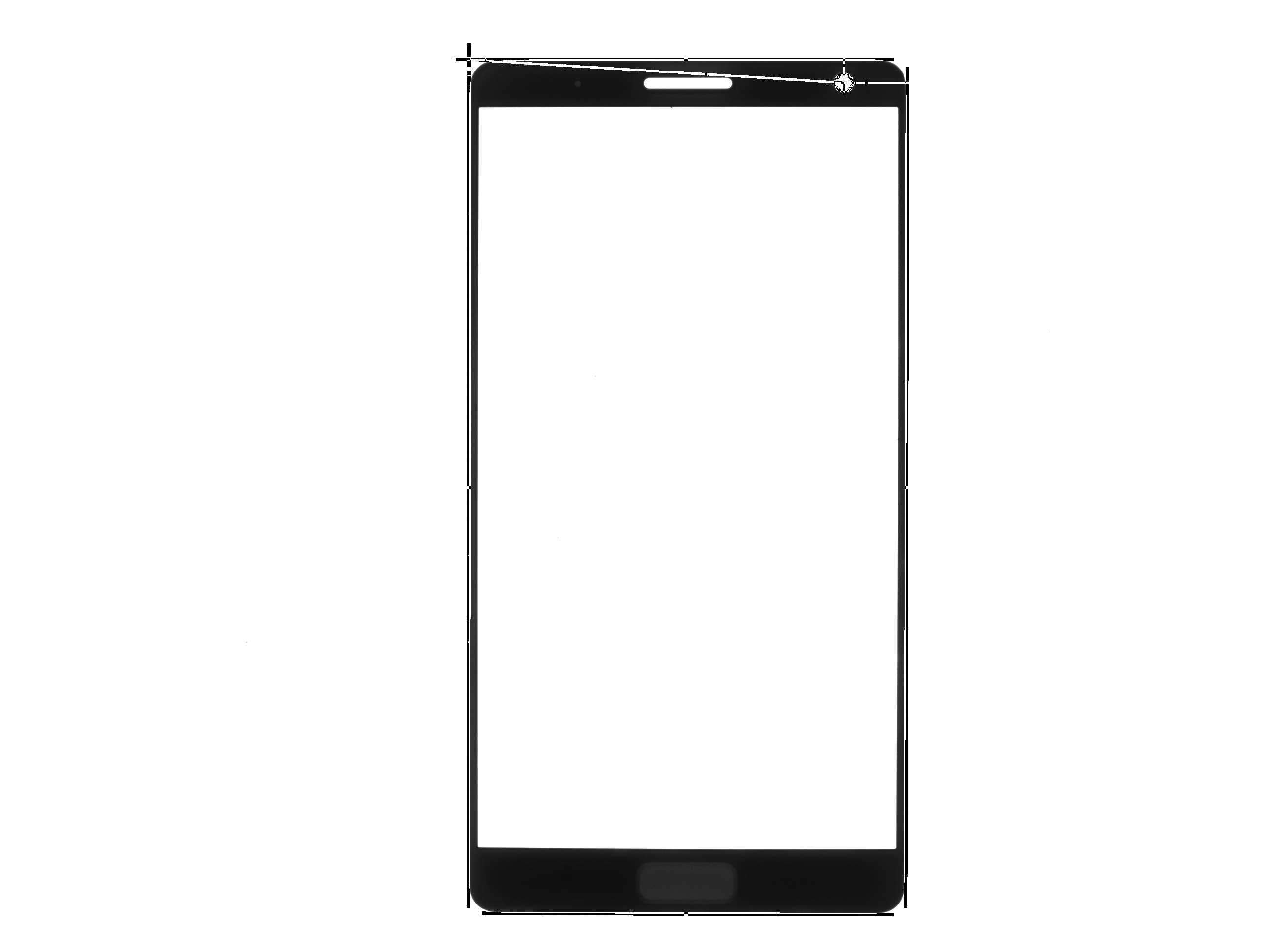
The “corner point” deserves an extra word. The four corners of this panel are genuine rounded fillets — there is simply no sharp corner pixel in the image to localize directly; the standard industrial practice is to define the corner as the virtual intersection of two fitted straight edges — it need not physically exist on the part, and the theoretical corner of a filleted part is still measurable. Each edge is averaged from dozens of edge points, and the intersection inherits their accuracy in full. This example runs the whole formula kit across the panel: the angle between the top and bottom short edges, the angle between the left and right long edges, the intersection of the top and left edges giving the top-left corner point, the camera hole center’s clearances to the top and right edges, the cross-part distance from the corner to the hole center, and the panel’s inner/outer width and height obtained from the mean of point-set-to-opposite-edge distances (Figure 21.2). All measured values are in Table 21.1.
| Geometric quantity | Measured | Note |
|---|---|---|
| Top–bottom edge angle (°) | 0.2365 | real non-parallelism (≫0.003° noise floor) |
| Left–right edge angle (°) | 0.0647 | real non-parallelism |
| Top⊥left right-angle error (°) | 0.0947 | 90°−89.9053°, top-left squareness |
| Top-left corner (px) | (957.475, 121.435) | virtual intersection of two edges |
| Hole center → top edge distance (px) | 47.769 | camera top clearance |
| Hole center → right edge distance (px) | 129.780 | camera right clearance |
| Corner → hole center distance (px) | 765.908 | cross-part point-to-point |
| Camera hole center (px) | (1721.930, 168.594) | center of 48-point circle fit |
| Camera hole radius (px) | 17.051 | fitted circle radius |
| Panel width L↔︎R (px) | 893.020 | mean of point-set-to-edge distances |
| Panel height T↔︎B (px) | 1744.362 | mean of point-set-to-edge distances |
The credibility of this table comes from geometric self-consistency: the pairwise angles measured among the four edges — 0.24° top–bottom, 0.06° left–right, 0.09° top⊥left right-angle error, 0.16° top⊥right — are all within a few tenths of a degree, confirming that the four independently fitted edges do enclose an approximate rectangle; the panel width of 893 px and height of 1744 px also agree with the dark-region silhouette span. The distance quantities are then real incoming dimensions: the camera hole’s top clearance of 47.8 px and right clearance of 129.8 px are exactly the critical gaps the camera aperture alignment must hold when such a panel is assembled. All readings stop in the pixel domain — converting to physical dimensions requires multiplying by the camera calibration scale factor (Chapter 5). It bears emphasizing: the geometric-measurement stage is exact formulas, and the uncertainty of every number in the table comes entirely from the edge-point noise \(\sigma_e\) propagated through fitting; the formulas themselves are word-perfect.
21.3 Parallelism, Roundness, and Straightness
Beyond dimensions, drawings carry another class of requirements, written in the frames of geometric dimensioning and tolerancing (GD&T). Their language is not “measure how much” but the tolerance zone: the toleranced feature must lie entirely within a region of given width — for parallelism the zone is between two lines parallel to the datum line, for straightness it is between two parallel lines, and for roundness it is the annulus between two concentric circles. The starting point of this language is assembly function: as long as the feature lies wholly within the zone, whatever its specific shape, assembly with the mating part is guaranteed. The universal recipe for evaluating them by vision measurement is one and the same: take the toleranced feature’s set of edge points, compute deviations against the evaluation datum, and max−min is the minimum zone width that contains the point set. The beauty of a real part is that these zone widths contain genuine form deviations, with no need to inject artificial defects.
Parallelism. With the fitted left long-edge line as datum, the max−min of the distances from the right long edge’s 90 edge points to the datum is 1.487 px (over a span of about 1060 px); with the top edge as datum, the bottom edge’s parallelism is 2.790 px (over a span of about 670 px). These two numbers can be read apart: the short edges’ parallelism comes almost entirely from that 0.237° real angle — \(670\times\tan(0.237^\circ)\approx2.77\) px, differing from the measured 2.790 px by only 0.02 px, with the remainder being the bottom edge’s own form undulation; of the long edges’ 1.487 px, the angle contributes \(1060\times\tan(0.0647^\circ)\approx1.20\) px, with the remaining ~0.29 px coming from the long edge’s own bow. Parallelism is the sum of systematic tilt and local form, taken as the max−min extreme, and it absorbs the datum line’s fitting error in full as well.
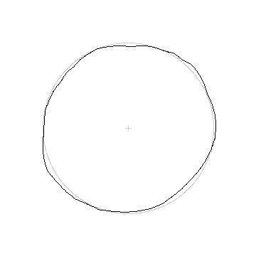
Roundness. Hole diameter and roundness are the most common judgment pair for assembly-class parts: the former determines the fit clearance, the latter whether aperture alignment and load are uniform. In this example, the max−min of the radial deviations of the camera hole’s 48 rim edge points from the fitted circle (radius 17.05 px) is 0.252 px — a real, tiny out-of-roundness, not a synthetic defect. Figure 21.3 plots the radial deviations magnified 60× on the nominal circle, and one can see the real rim is not perfectly circular: the deviation is dominated by low-order undulation (slight ovalization plus local bumps and dips), with the bottom and lower-left arcs bulging slightly outward. This “low-order dominated” out-of-roundness shape is the typical fingerprint of a stamping/laser hole-cutting process. A reminder about the datum’s role: the least-squares circle is the most stable to sampling noise, but its datum is pulled bodily by any local bump or dip, so the out-of-roundness “account” gets spread unevenly across the arcs — if some arc carries clear impact damage, the adjacent intact arcs end up bulging outward relative to the new datum and the arc directly opposite recedes inward (the industry case of Section 21.4 details a judgment dispute caused by exactly this).
ISO roundness evaluation admits several reference circles: the least-squares circle (LSC), the minimum zone circle, the minimum circumscribed circle, and the maximum inscribed circle. The minimum zone circle gives the smallest zone width by definition and is the very embodiment of the GD&T semantics; the least-squares circle is the most stable to compute and the least sensitive to sampling noise, but its zone width is systematically larger and its datum gets pulled by local defects. A reported roundness must state which one was used.
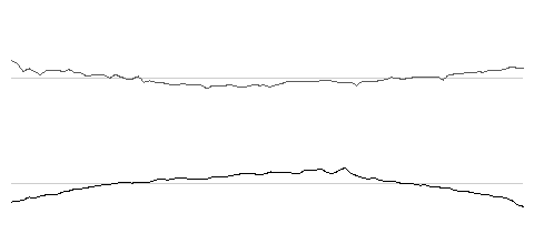
Straightness. The max−min of the left long edge’s normal deviations is 0.624 px, and the right long edge’s is 0.872 px (both 90 points, span about 1060 px). The deviation profile (×40) in Figure 21.4 shows the real shape of the two edges: the left edge (top) is fairly straight, with only small high-frequency undulation; the right edge (bottom) carries a gentle bow plus a local bump. Both are the part’s real edge form, with no artificial step — the right edge being more bowed also directly explains the “~0.29 px from edge form” portion of the left–right parallelism of 1.487 px discussed above.
Zone-width quantities are extreme-value statistics: the more points sampled, the larger the expected range of the noise, and max−min grows slowly with it — exactly the opposite of averaging-class quantities such as centers and angles, which get more accurate with more points. This is why inspection protocols for roundness and straightness must specify the number of sampling points; otherwise numbers from two machines are not comparable.
21.4 SciVision Implementation
The basic geometric quantities are provided by SCIMV::SciSvGeometryMeasure, each API corresponding to one formula of Section 21.2:
SCIMV::SciSvGeometryMeasure gm;
double angleDeg = 0, d = 0;
rc = gm.IncludedAngle(t1, t2, l1, l2, /*mode angle between lines*/1, &angleDeg);  // top⊥left squareness
rc = gm.PointToLineDistance(holeCenter, t1, t2, &d);                              // hole->top
SciPoint corner;
rc = gm.LinesIntersection(t1, t2, /*lineType line*/0, l1, l2, 0,
                          /*parallelThresh*/7, &corner);                          // virtual corner at fillet
double dMin = 0, dMax = 0; SciPoint pNear, pFar;
rc = gm.PointsToLineDistance(rightPts, l1, l2, &dMin, &dMax, &pNear, &pFar);
double width = 0.5 * (dMin + dMax);    // panel width (mean)
double parallelism = dMax - dMin;      // left|right parallelism zone width
Lines are uniformly represented by two endpoints (a pair of SciPoint). With mode=1, IncludedAngle returns the angle between lines, falling in [0°, 90°] — when the top and left edges are nearly perpendicular it returns about 89.9°, and the squareness is 90° minus that. In LinesIntersection, parallelThresh=7 is the parallelism-test threshold: when the two lines’ directions are too close, the intersection is ill-conditioned and the interface simply refuses to output one — in this example the top and left edges are nearly perpendicular, far from that threshold. PointsToLineDistance returns in one call the minimum and maximum point-set-to-line distances along with the corresponding points: the mean is the nominal distance to the opposite edge (panel width/height), and max−min is the parallelism zone width. The hole is located in one step by SciSvEllipseLocator::EllipseLocator, whose four output point arrays (fit/effective/rejected points) must all be passed as real entities, or rc=120001015.
Two engineering reminders. First, the Roundness/Straightness of SciSvGDTTools return normalized [0,1] scores (closer to 1 means “better”), not GD&T tolerance zone widths: this chapter measured a roundness score of 0.9964 for the camera hole; and the straightness scores of the left and right long edges are both 1.000000 — even though their real zone widths are plainly 0.624 px and 0.872 px, nearly 40% apart, the normalized score flattens the two into the same saturated value, leaving no way at all to set a threshold against a drawing callout like “straightness ≤0.02 mm”. Nor is there any published conversion formula between score and zone width; they can only serve as a relative trend reference among parts of the same type, and if you must use them for monitoring you first have to calibrate a “score-to-zone-width” curve from reference samples of known zone width. Zone-width values used for tolerance judgment are always computed as max−min from the point arrays yourself (which is where every number in this chapter’s text comes from). Second, the output distance array dstPtPositionArr of FitLine is not the signed perpendicular distance from each point to the line it returns; its semantics are opaque, so for straightness you must write your own “signed point-to-line distance” (devToLine) and take its range. One old pitfall is worth restating in passing: FitLine returns a degenerate result for strictly vertical point sets, so the left and right vertical long edges first swap x/y on all points, fit, and then swap the resulting line’s endpoints back. The complete project that generates all of this chapter’s images and numbers lives in code/geometric_measurement/.
Industry Case: The Roundness Evaluation Dispute
A bearing plant’s raceway roundness judgment once reached a deadlock: the customer’s incoming inspection used a roundness tester sampling thousands of points densely, evaluated by the minimum zone method; the production line’s vision system used a few dozen edge points, evaluated by the least-squares circle. One part, two numbers — the line’s value was systematically about 15% lower (sparse sampling misses peaks and valleys and pulls the reading down, an effect that outweighed the opposing effect of the least-squares datum’s systematically larger zone width), parts the line passed were rejected by the customer, and the two sides argued for months. The eventual resolution lay not in algorithms but in protocol: the inspection protocol explicitly recorded the evaluation method (minimum zone vs least squares) and the number of sampling points, and a calibrated conversion margin was set for the line’s values. The lesson takes one sentence: zone-width quantities like roundness and straightness have no “true value” detached from the evaluation method — a reported geometric quantity must be reported together with its evaluation method and sampling conditions.
21.5 Summary
- The measurement chain is “image → edge points → primitives → geometric quantities → judgment”: the geometric-measurement stage is exact formulas and introduces no new error; the final accuracy comes entirely from the edge-point noise \(\sigma_e\) propagated through fitting (\(1/\sqrt N\)); on the real panel this chapter measured edge-fit RMSEs of ≲0.1–0.28 px.
- Fix the noise floor first, then judge real signal: the long-edge direction error is \(\sigma_\theta\approx(\sigma_e/L)\sqrt{12/N}\approx0.003^\circ\); the measured left–right non-parallelism of 0.065° and top–bottom of 0.24° are both far above the noise floor, genuine part geometry rather than jitter.
- Virtual intersection measures the corner of a filleted part: the panel’s four corners are genuine rounded fillets, and the corner point is given by the virtual intersection of the top and left edges at (957.5, 121.4), inheriting the accuracy of each edge averaged over dozens of points.
- Zone-width quantities (parallelism/roundness/straightness) are extreme-value statistics with real shape: the left–right parallelism of 1.487 px splits into an angle contribution of 1.20 px plus 0.29 px of edge form; the camera hole’s real roundness is 0.252 px and the left/right long edges’ real straightness is 0.624/0.872 px — all from the part itself, with no synthetic defects.
- Recompute key quantities from the raw point arrays yourself: the SDK’s GD&T tools return normalized scores (two edges whose zone widths differ by 40% both score 1.000000), and
FitLine’s distance array is not the true perpendicular distance — numbers used for tolerance judgment must be computed from the points up.
For a systematic treatment of uncertainty analysis for geometric quantities and subpixel measurement, see the book by Steger et al. (Steger, Ulrich, and Wiedemann 2018). The parallelism, roundness, and straightness tolerances used in this chapter have their symbol language and tolerance-zone definitions fixed by geometric dimensioning and tolerancing (GD&T) standards: the international system is ISO 1101, which gives the rules for indicating and interpreting tolerances of form, orientation, location, and run-out (International Organization for Standardization 2017); the North American system is ASME Y14.5, an equally authoritative statement of the same semantics on engineering drawings (American Society of Mechanical Engineers 2018). The “dispute over the evaluation datum” that Section 21.3 and the industry case keep touching on — the least-squares circle and the minimum zone circle yielding different zone widths — is treated specifically in the form-error fitting literature; Moroni and Petrò compare the principles and costs of various minimum-zone fitting algorithms, a good entry point for connecting this chapter’s max-min zone widths to standardized evaluation methods (Moroni and Petrò 2008).