34 Photometric Stereo
The three-dimensional imaging of the previous chapters, whether laser triangulation (Chapter 30) or deflectometry (Chapter 35), measured the macroscopic height of a surface — how far a part protrudes, how deep it is dented. But industrial inspection often cares about something else entirely: which direction each point of the surface actually faces. The sharpness of a stamped character, the texture orientation of a frosted surface, the slope of a shallow defect — at root these are all questions of surface normal, and the normal is insensitive to absolute height. Photometric stereo is made precisely for this: the camera stays fixed, and we simply switch among several light sources of known direction, capturing one image at a time; the same point appears bright or dark differently under different illumination, and this variation in brightness encodes exactly its orientation. By solving the multiple images jointly, we can recover at every pixel both its normal and its albedo.
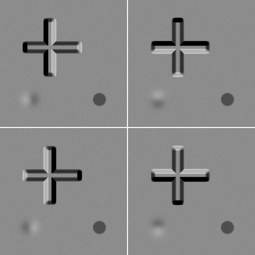
This technique also has a unique trick that is hard to replace elsewhere: it can cleanly separate “shape defects” from “appearance defects” into two distinct images. A dent changes the normal; a stain changes the albedo — a single-illumination grayscale image mixes the two together, whereas photometric stereo decouples them naturally. This chapter runs all its experiments on one synthetic relief board: a flat base plane carrying a raised cross-shaped logo, a 0.3 mm shallow dent defect, and a stain that alters only the albedo, not the height — exactly the “pair that ought to be separated” in inspection. Figure 34.1 shows the inputs captured under four illumination directions (slant angle 45°, azimuth 0°/90°/180°/270°).
34.1 The Lambertian Model and Solving for Normals
Photometric stereo is built on the Lambertian reflectance model (echoing the diffuse reflection of Chapter 4): the brightness of an ideal diffuse point depends only on the cosine of the angle between its normal \(\mathbf n\) and the incident light direction \(\mathbf l\), independent of the viewing direction:
\[ I = \rho \,(\mathbf n \cdot \mathbf l), \qquad \mathbf n \cdot \mathbf l > 0, \]
where \(\rho\) is the albedo of that point (how much it absorbs, how much it reflects), and \(\mathbf l\) is the unit lighting vector. Note that the unknowns come in two parts: the normal \(\mathbf n\) (two degrees of freedom, since \(\|\mathbf n\|=1\)) and the scalar \(\rho\) — three unknowns in all. A single image gives only one equation, far from enough; but if we capture one image under each of \(K\) light sources of known direction, we obtain \(K\) equations.
The key trick in solving is to combine \(\rho\) and \(\mathbf n\) into a single vector \(\mathbf g = \rho\,\mathbf n\), whereupon the equation becomes linear in the unknown: the \(k\)-th light source gives \(I_k = \mathbf g \cdot \mathbf l_k\). Stacking the \(K\) equations into the matrix form \(\mathbf I = L\,\mathbf g\) (each row of \(L\) is one light vector), \(\mathbf g\) is uniquely determined when \(K=3\) and the three light directions are linearly independent; when \(K\ge 4\) the system is overdetermined, and we solve the normal equations by least squares (echoing Chapter 2):
\[ \mathbf g = (L^\top L)^{-1} L^\top \mathbf I. \]
Once \(\mathbf g\) is solved, the decomposition is extremely clean — the magnitude is the albedo, the direction is the normal:
\[ \rho = \|\mathbf g\|, \qquad \mathbf n = \mathbf g / \|\mathbf g\|. \]
Why are 4 light sources better than 3? With 3 sources the solution is exactly determined, and any noise, any slight non-Lambertian behavior, enters the result undiminished; with 4 sources the system becomes overdetermined, and least squares averages across four measurements so that noise is partly canceled. The experiments of this chapter use 4 sources, with a full-image mean normal error of about 1.9°, already approaching the noise floor of \(\sigma=3\). One more source means one more measure of redundancy.
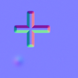
This chapter solves this small \(4\times 3\) system pixel by pixel. Encoding the normal as color by \(r=(n_x{+}1)/2\), \(g=(n_y{+}1)/2\), \(b=n_z\) yields Figure 34.2: the flat region appears blue because \(\mathbf n\approx(0,0,1)\), while the four side walls of the logo face different directions and take on red and green tints; the albedo image Figure 34.3 strips away the orientation information entirely, leaving only “how strongly each point reflects” — here the stain disk is a clear dark spot, while the dent defect is almost invisible. These two images come from the same set of data yet carry only “shape” and “appearance” respectively, which is exactly the protagonist of the next section.

34.2 Separating Shape from Appearance
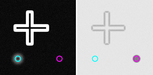
This is the killer-app experiment of photometric stereo. On the relief board we deliberately placed two utterly different kinds of defect: a 0.3 mm Gaussian dent (pure shape change, albedo unchanged) and a stain (pure albedo change, height unchanged). We take statistics over a small disk at each of three locations: a clean flat bottom as the baseline, the dent, and the stain. The results are in the table below, also corresponding to the left and right channels of Figure 34.4.
| Location | Normal deviation from vertical | Albedo |
|---|---|---|
| Flat-bottom baseline | 0.99° | 0.901 |
| Dent (0.3 mm) | 8.26° (8.3× the baseline) | 0.900 (−0.1%, unchanged) |
| Stain | 1.92° (near noise floor) | 0.500 (55% of the baseline) |
The numbers tell the story plainly: the dent shows up only in the normal channel — 8.26° against the 0.99° baseline is a jump of more than 8×, while its albedo does not budge; the stain shows up only in the albedo channel — the albedo drops to 55% of the baseline, while its normal deviation is only 1.92°, all but buried in the noise floor. Shape defects and appearance defects are sent by photometric stereo into two mutually non-interfering channels.
Why can 2D grayscale not do this? In a single grayscale image, a point may darken either because its albedo is low (a stain) or because its normal has tilted away from the light (a dent slope) — the two causes cannot be told apart within a single scalar. Photometric stereo uses multiple illumination directions to “stretch” this scalar into a vector equation, and magnitude and direction then part ways. This is exactly the root cause of single-illumination inspection repeatedly stumbling on “stains misjudged as dents.”
This bears directly on the design of decision criteria for defect detection (Chapter 26): shape-type defects (dents, scratches, edge collapse) should be thresholded on the normal or on curvature derived from the normal, while appearance-type defects (stains, oxidation, print smudges) should be thresholded on the albedo. The two kinds of defect require different criteria, and photometric stereo conveniently provides the two raw images that allow them to be judged separately.
34.3 Height Integration
With a normal field in hand, one naturally wants to integrate it back into height. The surface slopes corresponding to the normal \(\mathbf n=(n_x,n_y,n_z)\) are \(p=h_x=-n_x/n_z\) and \(q=h_y=-n_y/n_z\); solving the Poisson equation \(h_{xx}+h_{yy}=p_x+q_y\) then recovers the height (this is of the same origin as the frequency-domain integration of Frankot–Chellappa in Chapter 11, while this chapter solves it in the spatial domain by SOR iteration). The integrated height map is shown in Figure 34.5, and the experimental results are intriguing:
- Slowly varying features are recovered well. The 0.3 mm Gaussian dent integrates to −0.317 mm, less than 6% off the true value of −0.300 mm — smooth, shallow defects are exactly integration’s strong suit.
- Steep walls are severely underestimated. The raised logo has a true height of 2.00 mm, yet integration yields only 1.16 mm. The reason is honest and profound: the logo’s side walls, sloping at about 76°, undergo self-shadowing under a 45°-slant light, with the walls either facing away from the light or covered by their own shadow, so their normals are “flattened” by the solver and the step height decays accordingly. This is not a bug but a genuine teaching point of photometric stereo under steep geometry — it excels at microscopic slope but is poor at restoring near-vertical steps.
- Low-frequency drift. The four corners of the flat bottom should be at equal height, yet after integration the height spans 0.094 mm. This is the intrinsic low-frequency drift of Poisson integration under Neumann boundaries: integration constrains only slope (the derivative of height), and a global slow tilt leaves almost no trace in the derivative, so it cannot be pinned down.
Remember the boundary of photometric stereo’s height capability in one line: it excels at microscopic relief, not at absolute height. Slope information is its first-hand data; integration is only an after-the-fact reconstruction. The more high-frequency and slowly varying the relief (scratch depth, orange-peel texture), the more accurate it is; the more large-scale the absolute step height or overall warpage, the less reliable. For absolute height, go back to laser triangulation or deflectometry.

34.4 Lambertian Violations and Robustness
The Lambertian model is the bedrock of the whole solution, yet real surfaces are often non-Lambertian: metal, glaze, and oil films produce specular highlights, and protrusions cast shadows. A highlight is a bright spot far exceeding diffuse reflection, while a shadow is a dark region that should have had brightness but is zero — neither satisfies \(I=\rho(\mathbf n\cdot\mathbf l)\), and once one slips into the least-squares fit, it drags the entire solution of that pixel off course.
We add one more specular highlight region to the relief board and capture a 5th image containing the highlight, then compare the normal error of three solution methods in the highlight region:
| Configuration | Normal error in highlight region |
|---|---|
| 4 lights (no highlight) | 1.15° |
| 5 lights (with highlight, naive least squares) | 11.81° |
| 5 lights (with highlight, robust rejection) | 1.15° |
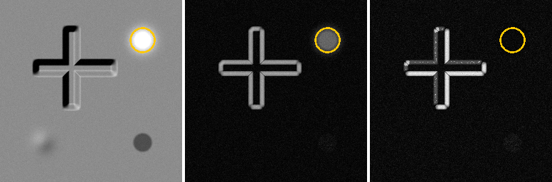
Naive least squares treats that highlight measurement as trustworthy data, and the error explodes from 1° to nearly 12°. The approach of robust photometric stereo is extremely simple yet effective: first solve once using all measurements, find the term with the largest residual (most likely the highlight or shadow), reject it, and re-solve with the remaining measurements. In this way the error falls back to 1.15° — on par with the case of no highlight at all. The error maps in the middle (naive least squares) and on the right (robust rejection) of Figure 34.6 intuitively contrast the night-and-day difference between the two in the highlight region.
The recipe of robust photometric stereo can be condensed into one phrase: more light sources + outlier rejection. This is of the same origin as Huber robust line fitting in Chapter 14 — both acknowledge that “a few measurements are outliers” and use rejection or down-weighting to exclude them from the estimate. The only difference is that there the outliers came from defect edges, while here they come from highlights and shadows. The more light sources, the more redundancy available for rejection, and the stronger the robustness.
34.5 SciVision Implementation
To state it honestly: SciVision’s photometric stereo interface SciSvPhotometricStereo::CalibratedPhotometricStereo produces silent empty output on this machine — it does not crash, returns code rc=0, but the Nx/Ny/Nz/albedo outputs are all 0×0 empty images, and it prints “Directory does not exist.” to stderr (exactly the same failure signature as PhaseMeasure in Chapter 35, suspected to be a missing runtime resource directory). This chapter therefore records the defect faithfully with a subprocess probe, and switches the entire solution to a hand-written per-pixel least squares — which is exactly the mathematical substance of Section 34.1. The core snippet follows.
// Per-pixel solve g = albedo·n: min_g Σ_k (I_k − g·l_k)²
//   normal equation (Σ l_k l_kᵀ) g = Σ I_k l_k
double M[9] = {0}, b[3] = {0};
for (int k = 0; k < K; ++k) {                 // K light sources
    double l[3] = { Lx[k], Ly[k], Lz[k] };    // known light directions
    for (int r = 0; r < 3; ++r) {
        b[r] += I[k] * l[r];                  // Σ I_k l_k
        for (int c = 0; c < 3; ++c)
            M[r*3 + c] += l[r] * l[c];         // Σ l_k l_kᵀ
    }
}
solve3(M, b, g);                              // solve 3×3 for g
// Robust: reject the term with the largest residual, then re-solve with the remaining ≥3 terms (remove highlight/shadow)
if (robust && K >= 4) {
    int worst = argmax_k |I[k] − g·l_k|;
    re-accumulate M,b (skipping worst), then solve3 -> g;
}
double albedo = norm(g);                      // magnitude = albedo
n = g / albedo;                               // direction = normal (take n_z≥0 facing the camera)
Height integration is implemented by per-point SOR iteration of the Poisson equation: compute the slopes \(p,q\) from the normals, take their divergence to obtain the right-hand side \(f=p_x+q_y\), then iterate with relaxation factor \(\omega=1.9\) to solve \(h_{xx}+h_{yy}=f\) (Neumann boundary). The complete runnable project is at code/photometric_stereo/.
Industry Case: Stamped Characters and Stains on Nameplates
A metal-nameplate inspection line had to judge two things at once: whether the stamped characters were clear and complete (shape-type), and whether the surface was contaminated by oil stains or oxidation spots (appearance-type). The early single-illumination grayscale scheme made the shadow at the bottom of a stamp and a dark oil stain both appear as “dark regions” in the image, hard to tell apart — raising the threshold missed shallow stamps, lowering it misjudged oil stains as character defects, and the false-detection rate stayed high. Switching to 4-light photometric stereo resolved the problem at once: the normal map reflects only the stamping depth and edge steepness of the characters, while the albedo map reflects only the reflectance change of oil and oxidation. The two maps each set their own criteria, without mutual interference, and the false-detection rate dropped sharply. The lesson is clear: when “defects” include both shape-type and appearance-type, photometric stereo’s ability to decouple the two into separate channels is irreplaceable — something no single-illumination scheme can deliver.
34.6 Summary
- Photometric stereo measures the normal, not the height. The camera stays still while light sources of known direction are switched; the Lambertian model \(I=\rho(\mathbf n\cdot\mathbf l)\) resolves the brightness variation into each point’s orientation; 3 sources fix the solution, 4+ sources give least squares, and the magnitude of \(\mathbf g=\rho\mathbf n\) is the albedo while its direction is the normal.
- It can separate shape defects from appearance defects. In this chapter’s experiments the dent jumps to 8× the baseline in the normal channel while its albedo stays unchanged, and the stain pushes the albedo down to 55% while its normal does not move — a decoupling that single-illumination grayscale cannot achieve, and one that directly decides which channel the defect criterion should be built on.
- Normals can be integrated back into height, but with limits. Slowly varying shallow defects are recovered accurately (dent −0.317 vs −0.300 mm), steep walls are underestimated due to self-shadowing (logo 1.16 vs 2.00 mm), and low-frequency drift is an intrinsic product of the Neumann boundary — good at microscopic relief, poor at absolute height.
- Robustness = more light sources + outlier rejection. Highlights and shadows violate the Lambertian assumption, naive least squares explodes in error (11.81°), and after rejecting the measurement with the largest residual the error falls back to 1.15°, of the same origin as Huber robust fitting.
- The SDK’s photometric stereo interface is unusable on this machine (silent empty output), and the hand-written per-pixel least squares is both the fallback and the very substance of this chapter’s mathematics.
The foundational work of photometric stereo is Woodham’s method of determining surface orientation from multiple illuminations (Woodham 1980); to address highlights and shadows that break the Lambertian assumption, Wu et al. model the problem as low-rank matrix completion and recovery, giving a convex-optimization solution for robust photometric stereo (Wu et al. 2011) that shares its spirit with this chapter’s outlier rejection. A systematic treatment of photometric stereo, shape reconstruction, and robust estimation in industrial vision can be further consulted in the book by Steger et al. (Steger, Ulrich, and Wiedemann 2018).