26 Defect Detection
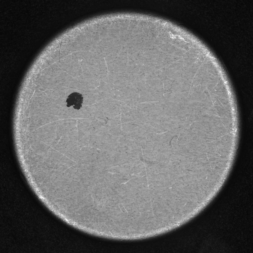
The previous three chapters of the inspection part handed you three tools: blob analysis (Chapter 23) segments and measures regions from a binary image, contour analysis (Chapter 24) reconciles an actual contour against a theoretical one point by point, and shape features compress “what it looks like” into comparable numbers. But all of them answer “what is this thing, how big is it, how far is it off” — while the most common question on a production line is a different one: “does this product have anything it shouldn’t have?” Contamination, foreign objects, scratches, edge chips, burrs… defect morphologies can never be enumerated exhaustively, and you cannot write a detector for each one. This chapter presents the paradigm that closes out the entire inspection part: a defect is a deviation from “normal.” The problem is thereby inverted — rather than defining the endlessly varied defects, first define the one and only “normal.” Following the thread of “where does normal come from,” industrial defect detection splits into three routes: reference comparison — build a reference from good samples and compare pixel by pixel (the variation model, this chapter’s protagonist); rule-based judgment — describe the acceptance condition with geometric rules, such as “edge straightness must not exceed 2 px” (edge-defect and contour-defect detection); statistical outlier detection — rely on no external reference at all and find statistically anomalous regions within the image itself. The chapter runs all experiments on a set of real industrial sample images: 5 frames of 2448×2048 8-bit grayscale from Smart3’s “scratch-inspection example recipe” (Figure 26.1), each a fibrous filter disk (disk surface gray level about 150, dark background about 80), with real scratches scattered across the surface and each carrying one class of real defect — a large dark contamination, a bright foreign object, an edge chip. It is precisely this set of “no clean master, only real parts” samples that forces out several lessons the variation model never gets to learn in an idealized synthetic scene.
26.1 The Variation Model: Let the Samples Define Normal
The naive approach to filter inspection is to subtract a golden-sample image from the image under test and threshold the difference. It fails immediately: the disk surface is a random fiber texture, and the fiber orientation differs on every disk; even between two good parts, subtracting pixel by pixel sprouts “defects” at every fiber and every scratch. The insight of the variation model is this: normal is not a single image but a band; and the width of the band should not be dictated by an engineer’s gut feeling — it should be set by the variation of the training samples themselves.
For \(n\) good training images, compute the per-pixel gray-level mean \(\mu(x,y)\) and standard deviation \(\sigma(x,y)\); the acceptance interval for that pixel — the tolerance band — is then
\[ \big[\,\mu - \max(a,\ k\sigma),\ \ \mu + \max(a,\ k\sigma)\,\big], \]
where \(a\) is the absolute threshold and \(k\) is the variation threshold coefficient. The \(k\sigma\) term lets the tolerance adapt to each pixel’s true variation; \(a\) is the floor — in regions where \(\sigma\) is close to zero, a \(\sigma\) estimated from only a few samples is itself unreliable, and the absolute lower bound keeps the tolerance band from collapsing to zero width and flagging pure noise as defects. At inspection time, any test pixel that falls outside the band is marked as a defect pixel. The model itself is just two images: an upper-bound image and a lower-bound image.
But this set of real samples drives the variation model’s prerequisites straight into a wall. The textbook variation model carries a hidden assumption: the \(n\) good images must be pixel-wise repeatable — the same coordinate sees the same structure on every good part, and the only difference comes from process variation (registration jitter, ink quantity, illumination). A printed label satisfies this; a loose fibrous filter disk does not: register the 5 disks by centroid (translate to center, normalize intensity) and train the SDK variation model, and the texture simply does not line up at the pixel level — the per-pixel \(\sigma\) is blown up by texture misregistration, and the result reports nearly a thousand texture false-alarm regions on every disk, including the cleanest golden sample (Section 26.2 gives the measured 692–1459). This is the first lesson the real samples teach: the registered golden-sample variation model needs a “repeatable appearance,” and it cannot handle non-repeatable textures such as fibers, fabric, or matte surfaces.
“Repeatable appearance” is the invisible threshold of the reference-comparison route. Print, labeling, screen printing, and molded-part surfaces are pixel-wise repeatable after registration — the variation model’s home turf — while fiber paper, nonwovens, brushed metal, and frosted surfaces are pixel-wise random, and cross-sample registration only bakes texture misregistration into the tolerance band. To judge whether a surface can use a registered variation model, ask one question first: register two good parts and subtract — is the difference image flat, or covered in texture?
The way out is to change where “normal” comes from: not across samples, but within the same image. For each disk, its own surface is slowly varying at the large scale (bright center, rim halo, overall flat field), and local anomalies are the defects. So the “normal model” \(\mu\) is taken as that disk’s own large-window smooth background (a disk-masked box mean of radius 150 px), which erases scratches and contamination and keeps only the slow illumination; the \(\sigma\) in the band width is taken as the robust scale of the golden sample’s residual, \(1.4826\cdot\mathrm{MAD}=8.69\) (the normal noise level of the disk’s fiber texture), with a floor \(a=10\). Detection then lands on the residual \(R=I-\mu\): \(|R|>\max(a,k\sigma)\) is a defect. This is still the same variation-model band mathematics, only with \(\mu\) from spatial smoothing and \(\sigma\) from the golden texture — it sits at the intersection of the “reference comparison” and “statistical outlier” routes.
One engineering trick is worth pointing out: disk segmentation uses Otsu, and the core of the dark contamination is darker than the threshold, so it is assigned to the background, leaving a hole in the disk mask. The smooth background therefore takes the surrounding bright fiber values at the hole (in the mean image of Figure 26.2 (b) the contamination has been “filled bright” into a clean surface), so the residual at the hole is strongly negative — the contamination hole is cleanly exposed by this very mechanism as a large negative-residual defect (the variation image of Figure 26.2 (c)).
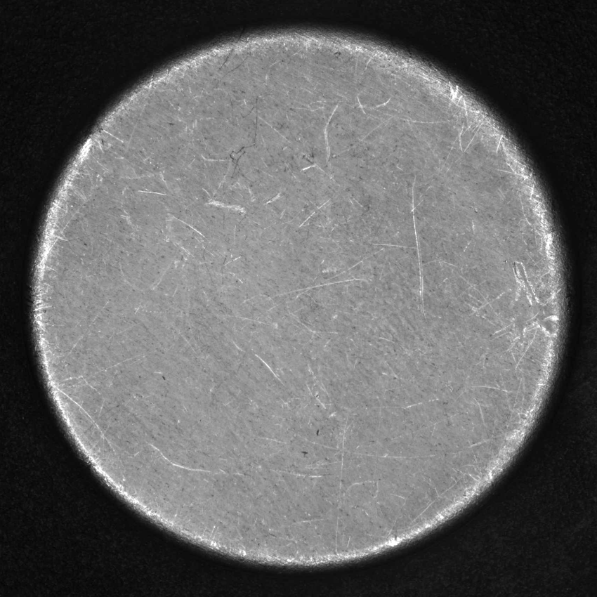
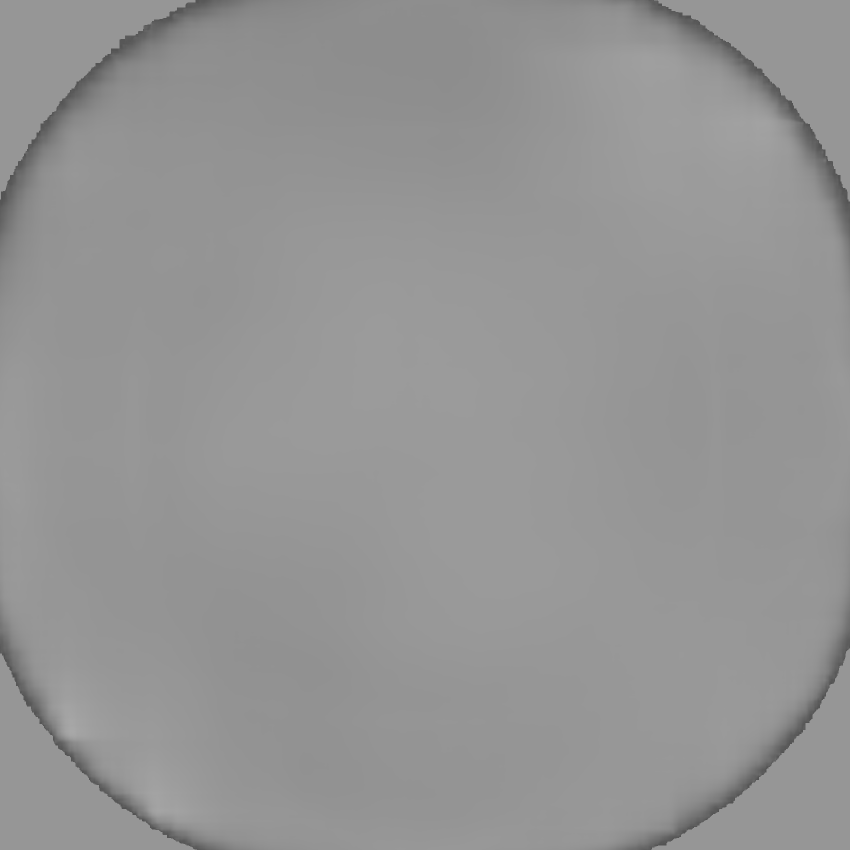
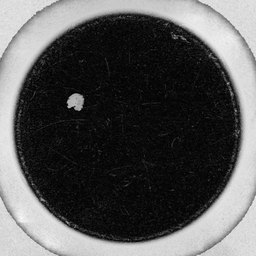
interiorR circle.
26.2 Detection Experiments
First put the measured failure of the registered multi-sample SDK variation model on the table. Take the three disks with clean interiors — 003, 004, 005 — as good references (their real defects are at the edge and are excluded by an interior circular mask), register by centroid and normalize intensity, then train the SDK variation model (\(a=12\), \(k=3\)) and compare disk by disk:
| Test disk | 001 | 002 | 003 | 004 | 005 (golden) |
|---|---|---|---|---|---|
| Defect regions | 1017 | 1298 | 692 | 1459 | 1094 |
Golden sample 005 is one of the model’s own training images, yet it is still reported with 1094 “defects,” which nails the problem down: it is not a poorly tuned threshold but the fact that the prerequisite of pixel-wise repeatability does not hold. Switching to the self-reference band of Section 26.1, detection immediately becomes readable. At the normal setting (\(k=5\), band width \(\max(10,5\times8.69)\approx43\), minimum connected component 30), detecting disk by disk and counting separately by polarity (dark defect / bright scratch):
- 002 dark contamination: detected dark-defect area 9811 pixels, largest connected component 9738 pixels, mean contrast −101 gray levels — a contamination blob nearly 10,000 pixels in size and 100 levels darker than the surface, at position (504, 676) (Figure 26.3 (a)). It is the strongest, most unambiguous real defect of the whole set.
- 001 foreign object: a curled bright fiber object embedded on the surface — the bright part detected (largest connected component contrast +93 gray levels) and its dark shadow detected at the same time (dark-defect area 2960, largest 2771, contrast −82); both polarities cross the band (Figure 26.3 (c)).
- 005 golden sample: dark-defect area only 343 pixels (no contamination), but the real scratches on the surface are detected as 2934 bright pixels (Figure 26.3 (b)) — “clean” for a golden sample is only relative; it too is covered with scratches.
- 003 / 004: interior dark-defect areas 480 / 440 (minor); their real defect is an edge chip, which falls outside the interior detection circle and is handled by the rule-based route (Section 26.4).
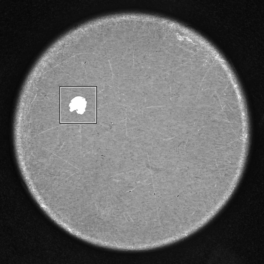
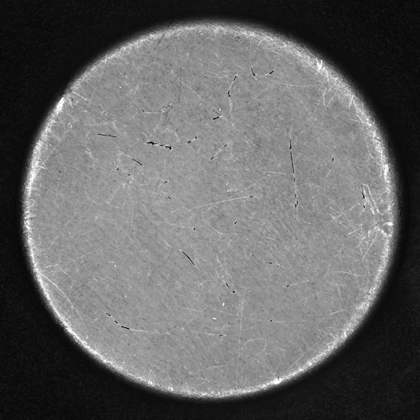
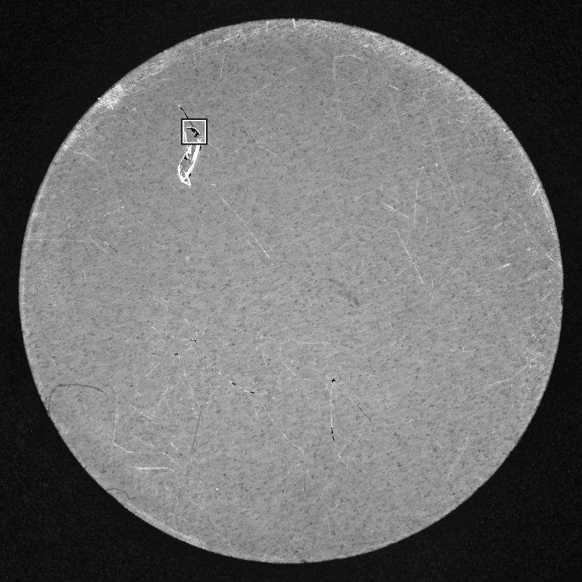
Case 002 confirms the robustness of the self-reference route: the contamination blob is a hundred gray levels darker than the surface, far from the noise tail, and crosses the band solidly regardless of how tight or loose the threshold is. The scratches of 005, on the other hand, demonstrate the other extreme — they are only ten to a few tens of gray levels brighter than the surface, hugging the noise tail, the real battleground of threshold tuning.
26.3 The Threshold Dilemma
The normal setting of \(k=5\) did not fall from the sky. Sweeping the same self-reference model and the five disks across tight (\(k=3\), band ≈26), normal (\(k=5\), ≈43), and loose (\(k=8\), ≈70) settings (floor \(a=10\), minimum connected component 30), the detected areas split by polarity are as follows (hand-written deterministic band, cross-validated against the SDK output in Section 26.5):
| Disk (defect) | Dark tight | Normal | Loose | Bright tight | Normal | Loose |
|---|---|---|---|---|---|---|
| 001 bright foreign object | 5939 | 2960 | 1935 | 4984 | 864 | 179 |
| 002 dark contamination | 12065 | 9811 | 9133 | 4592 | 241 | 0 |
| 003 edge chip | 5228 | 480 | 0 | 8729 | 1552 | 74 |
| 004 edge chip | 4168 | 440 | 109 | 13345 | 1520 | 163 |
| 005 golden sample | 2204 | 343 | 35 | 13384 | 2934 | 236 |
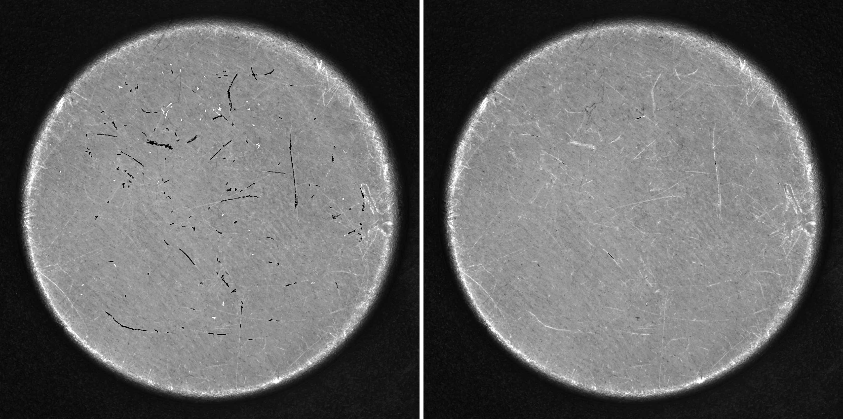
The differing fates of the two defect classes in the table are precisely the fundamental dilemma of defect detection. Dark contamination and foreign objects pierce through all thresholds: the dark defect of 002 barely changes from 12065 at the tight setting to 9133 at the loose, and the 001 foreign object holds from 5939 to 1935 — their contrast is strong enough that they are the “must-catch” real defects. Scratches and grains, by contrast, are extremely threshold-sensitive: the bright detection of golden sample 005 collapses from 13384 pixels at the tight setting to 236 pixels at the loose, and the bright scratches of 003 and 004 also decay by orders of magnitude. Figure 26.4 puts the two extremes of 005 side by side: in the left image (tight) the surface is densely covered with detected fine scratches and fiber grains — if scratches are an acceptable cosmetic blemish, these are false alarms; in the right image (loose) the frame is nearly clean, leaving only the deepest few scratches.
This is exactly where real samples are more honest than a synthetic scene: there is no “clean good part” here — every disk has scratches, and the boundary between “defect” and “blemish” is decided by the acceptance criterion, not by physics. The engineering procedure for tuning is a squeeze from both ends: first, on a set of disks judged “acceptable,” tighten the threshold until acceptable blemishes (shallow scratches) just stop being reported and false alarms are pressed to the permitted PPM level — this gives the lower bound; then verify detection on the known must-catch real defects (contamination, foreign object, chip) — this gives the upper bound. Between the two bounds lies the working window — and if the window does not exist (the shallowest must-catch defect and the acceptable blemish are inseparable in gray level), what needs changing is not the threshold but the imaging setup: lighting angle, spectral band, or resolution (the dark-field/bright-field choice of Chapter 4 is often made precisely to pry this window open).
This is isomorphic to the lesson of Chapter 7: a threshold’s “automatic” merely automates the act of picking a threshold and does not guarantee a fit to your scene. The variation model’s “automatic tolerance” is the same — \(k\sigma\) automatically adapts to the texture noise present in the golden sample, but “which deviation counts as a defect” is still an artificial line that must be drawn by the acceptance criterion, and “automatic” is no exemption from inspection.
26.4 The Rule-Based Route: Edge and Contour Defects
The self-reference variation model excels at contamination, foreign objects, and scratches inside the disk surface, but it cannot reach the edge chips of 003 and 004 — they fall outside the interior detection circle and are essentially the disk’s contour deviating from the circle it should be. When the acceptance condition can be written down as geometric rules (for instance, “the edge should be a circle of radius 760”), SciVision provides two modules on the rule-based route, introduced here as reconnaissance (not demonstrated in this chapter).
Single-edge defect detection (SingleEdgeDefectDetection, manual 8.11) targets requirements of the form “an edge should be straight/smooth”: along a set of search lines it extracts point pairs from the standard edge and the actual edge, computes the distance and angle deviation for each pair, and judges NG when a threshold is exceeded. It is essentially caliper-style (Chapter 20) line-by-line measurement plus limit checking, suited to local single-edge anomalies such as burrs on stamped parts, chipped blade edges, and nicks in sealing strips — exactly matching the edge chips of disks 003 and 004 in this set: take the disk’s theoretical circle as the standard edge, and where the actual edge dents inward beyond tolerance is a chip, no golden sample needed.
Contour defect detection (ContourDefectDetection, manual 8.14) compares the actual contour against a template contour as a whole and, beyond out-of-tolerance flagging, provides defect classification: breaks, dents, bulges, and fine burrs. It also supports width-defect detection between contour pairs and can generate a dispensing trajectory from the template — a set of capabilities plainly aimed at glue dispensing/coating inspection: whether the glue path has gaps (breaks), glue pile-up (bulges), insufficient glue (dents), and whether the glue width is in spec (contour-pair width). It belongs to the same family as the contour comparison (ContrastContour) of Chapter 24: the latter outputs a continuous deviation curve, the former directly outputs a classified defect list.
The division of labor between the two routes fits in one sentence: with a geometric prior and writable rules, take the rule-based route; with repeatable samples but no writable rules, take the variation model. The “normal” of the disk’s fiber texture cannot be described by a few geometric constraints, nor reproduced by cross-sample registration, and can only rely on single-image self-reference statistics; conversely, the disk’s edge “should be a circle of radius 760” is one clean rule, and there is no reason to train a model for it.
26.5 SciVision Implementation
The variation model is provided by SCIMV::SciSvVariationModel, with one interface each for training and comparison:
SCIMV::SciSvVariationModel vm;
SciImageArray trainImgs; // good training images (must be pixel-wise repeatable)
SciROIArray maskArr; // per-image mask regions (GenCircle for the disk interior)
SciROI trainRoi; // training region
SciImageArray model; // output: [0] upper bound 8U [1] lower bound 8U [2] reserved [3] mean 32F
long rc = vm.TrainModel(trainImgs, maskArr, trainRoi,
/*absThreshold*/ 12.0f, /*varThreshold*/ 3.0f, &model);
SciImage result; SciContourArray contours;
SciVarArray lengths; SciPointArray centers;
SciROI roi; // UNDEF = compare the whole image (circular ROI rejected, see below)
rc = vm.CompareModel(testImg, model, roi, /*minLength*/ 30, /*maxLength*/ 100000,
&result, &contours, &lengths, ¢ers);absThreshold and varThreshold are the \(a\) and \(k\) of the formula in Section 26.1. The key finding of this chapter on the real samples is that registered multi-sample training is unusable on the fibrous surface (Table 26.1; the golden sample itself reports 1094 false-alarm regions). The way out is to treat CompareModel as a generic “out-of-band pixel → contour extraction → length filtering” engine, feeding it a per-image self-synthesized self-reference model — model[3] holds that disk’s smooth background \(\mu\), model[0]/[1] hold \(\mu\pm\max(a,k\sigma)\), and model[2] is zeroed. This both sidesteps the registration prerequisite and reuses the SDK’s contour and length filtering. Measured cross-validation (band width 43, \(k=5\)):
CompareModel engine (self-reference synthesized model) against the hand-written band: the total defect-pixel counts agree (002: 9926 vs 10052), differing only in region granularity due to different connectivity rules.
| Disk | SDK comparison output (interior nonzero px / regions) | Hand-written band (area / regions) |
|---|---|---|
| 002 contamination | 9926 / 100 | 10052 / 9 |
| 001 foreign object | 3666 / 46 | 3824 / 18 |
| 005 golden sample | 2768 / 184 | 3277 / 54 |
This family of interfaces exposed several pitfalls in testing that must be recorded faithfully:
minLengthmust be ≥1: passing 0 returns error 120001014, even though the documentation states a valid range of [0, 100000].maxLengthmust be ≤100000: passing 1000000 returns error 120001015 (counter to the intuition of an “upper bound on length filtering,” and undocumented) — a new pitfall measured in this chapter.- All four output parameters must be given real objects: passing
NULLfor any one of them crashes outright (0xC0000005), even if you do not care about the contours or centers. CompareModeldoes not accept a circular ROI: passing an ROI generated byGenCirclereturns 120001015 (whereasTrainModel’s mask accepts circular ROIs); the comparison can only use a UNDEF/rectangular ROI, and restricting to the disk interior must be done by post-processing with a circular mask.- Registered multi-sample training fails on non-repeatable textures: see Table 26.1; the variation model’s per-pixel \(\sigma\) treats cross-sample texture misregistration as “process variation,” and the golden sample itself is flooded.
These pitfalls shaped this chapter’s experimental methodology: the threshold sweep and polarity statistics all use a hand-written \(\mu\pm\max(a,k\sigma)\) model (32-bit float, fully deterministic), cross-validated against the SDK CompareModel output — contamination 9926 vs 10052 for 002, foreign object 3666 vs 3824 for 001, the total defect-pixel counts agreeing, confirming the two implement the same mathematics. This continues the golden-experiment methodology of Chapter 5: what the documentation describes is a promise; what a controlled experiment with known behavior verifies is the truth — and when some kind of data invalidates one prerequisite of a commercial library, let your own hand-written mathematical reference serve as the arbiter. The complete project lives at code/defect_detection/, with the full measurement log preserved in the file headers.
Industry Case: Mistaking the “Golden Sample” for a Cure-All
A nonwoven filter-material inspection line copied print-inspection experience and tried to do surface defect detection with a registered variation model: it collected twenty “good” images to build the model, formed the band from per-pixel mean and variance, and went live with a false-alarm rate over 30%, nearly every frame flooded with small regions. Investigation found the root cause lay not in the threshold, not in the lighting, but in the fiber texture of the filter material being random from frame to frame and not lining up at the pixel level after registration — the variation model treated texture misregistration as process variation, and the tolerance band was stretched until it either false-alarmed everywhere or let real defects through. The final solution abandoned cross-sample registration and switched to single-image self-reference: each image is compared against its own large-window smooth background, with the band width set by the robust scale of that image’s texture. The lesson: the variation model has an invisible threshold — pixel-wise repeatability after registration. Print, labeling, and screen printing satisfy it; fiber, fabric, frosted, and brushed surfaces do not. Before going live, do a “register two good parts and subtract” health check first: if the difference image is covered in texture, stop counting on a registered golden sample and switch to a self-reference or texture-statistics route.
26.6 Summary
- The paradigm of defect detection is definition by inversion: defect morphologies cannot be enumerated; the operational definition is “a deviation from normal” — first define normal, then quantify the deviation. Normal can come from registered good parts (the variation model), geometric rules (edge/contour defects), or within-image statistics (self-reference).
- The registered variation model has an invisible threshold: pixel-wise repeatability. Real fibrous filter disks do not satisfy it — register 5 disks and train, and even the golden sample itself is flooded with 1094 texture false-alarm regions. Print-like surfaces are its home turf; fiber/fabric/frosted surfaces are not.
- The way out is a single-image self-reference band \(|I-\mu|>\max(a,k\sigma)\): \(\mu\) taken as the image’s own large-window smooth background, \(\sigma\) as the robust scale of the golden sample’s residual (8.69). It cleanly exposes the contamination hole (assigned to background by Otsu, filled bright by the smooth background) as a large negative-residual defect — the contamination blob of 002 at 9738 pixels, contrast −101 gray levels.
- Tune thresholds by squeezing from both ends: acceptable blemishes press false alarms to give the lower bound (golden-sample scratches 13384 at the tight setting → 236 at the loose), known must-catch real defects verify detection to give the upper bound (contamination pierces through all thresholds). On real samples the line between “defect” and “blemish” is decided by the acceptance criterion, not by physics.
- Every prerequisite of a commercial library must pass a golden experiment: the SDK
CompareModelwas repurposed as a self-reference detection engine and only after cross-validation against the hand-written band (9926 vs 10052) was confirmed to be the same mathematics; testing also forced out new pitfalls —maxLength≤100000, circular ROI rejected — documentation is a promise; the experiment is the behavior.
And so the inspection part closes: blob analysis gave us “segment and measure,” contour analysis gave us “point-by-point reconciliation,” shape features gave us “a language for shape,” and this chapter distills them all into the paradigm of “define normal, detect deviation” — and uses a set of real filter-disk samples to prove that when the paradigm meets the ground, the first thing that matters is asking the right question: where does “normal” come from? A map of methods for textured-surface defect detection can be found in Xie’s review (Xie 2008), which systematically organizes the statistical, structural, filter-based, and model-based routes around texture analysis; the canonical source for texture-feature statistics remains Haralick et al.’s GLCM paper (Haralick, Shanmugam, and Dinstein 1973); and for the frequency-domain (Fourier) route not pursued in this chapter, Tsai and Hsieh’s defect detection for directional textures is a clean exemplar (Tsai and Hsieh 1999). For a more systematic engineering treatment of industrial defect detection (including textured surfaces and extensions of the variation model), see the book by Steger et al. (Steger, Ulrich, and Wiedemann 2018).