8 Morphology

The output of thresholding (Chapter 7) is never a clean binary image. However well the threshold is chosen, the foreground is always left with a few pepper-like small holes, burrs hanging off the edges, two targets that should be separate glued together by a thin bridge, one target that should be whole split into pieces by a thin gap, and isolated noise dots scattered across the background. To the human eye these blemishes are trivial; to a program they are a disaster: the downstream blob analysis (Chapter 23) will count every noise dot as a target, count two merged targets as one, and count one fractured target as three. Mathematical morphology is the wrench that repairs binary images — it slides a small template across the image and, following the rules of set operations, deletes or fills in pixels, trimming the segmentation result into shapes the downstream algorithms can digest directly.

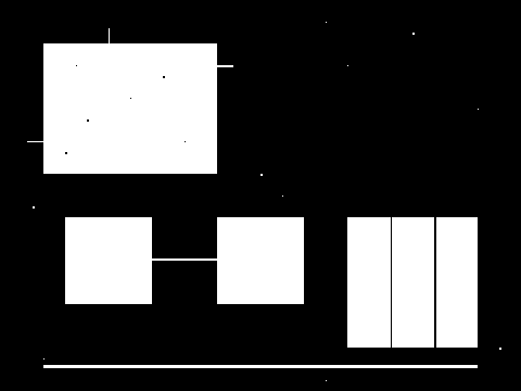
Throughout this chapter a single 480×360 synthetic binary scene runs through all the experiments (Figure 8.1). Every blemish in the scene is placed deliberately: a solid rectangle with 1–2 px pepper holes inside and 1–2 px burrs on its edges; two blobs merged by a 2 px thin bridge; a rectangle split into three pieces by 1 px and 2 px thin gaps; a 3 px-thick thin strip; plus 10 isolated noise dots (six 1×1 and four 2×2). All coordinates are hard-coded with no random numbers, so the statistics are identical on every run: 47426 foreground pixels in total, forming 16 blobs under 8-connectivity.

Figure 8.1: The synthetic binary scene used throughout this chapter: a rectangle with pepper holes and burrs, a double blob merged by a 2 px thin bridge, a rectangle split by 1 px/2 px thin gaps, a 3 px thin strip, and 10 isolated noise dots. Foreground 47426 px, 16 blobs under 8-connectivity.

8.1 Structuring Elements, Erosion, and Dilation

Every morphological operation revolves around one protagonist: the structuring element. It is a small shape template with an anchor — most commonly a 3×3 or 5×5 rectangle with the anchor at the center. During the operation the anchor scans the image pixel by pixel, and the neighborhood covered by the structuring element decides that pixel’s fate. The structuring element is to morphology what the convolution kernel is to linear filtering (Chapter 6): the template’s shape and size determine the operation’s entire character.

The two most basic operations form a pair of “antonyms.” Erosion is defined in set terms as

\[ A \ominus B = \{\, z \mid B_z \subseteq A \,\}, \]

where \(A\) is the set of foreground pixels and \(B_z\) denotes the structuring element \(B\) translated so that its anchor sits at position \(z\). In one sentence: the anchor position stays foreground only if the structuring element fits entirely inside the foreground. Anywhere that cannot accommodate the structuring element — thin bridges, burrs, isolated small dots, the outermost ring of every target — is stripped away. Dilation is the opposite:

\[ A \oplus B = \{\, z \mid B_z \cap A \neq \emptyset \,\}, \]

as long as the structuring element touches the foreground in even one pixel, the anchor position is set to foreground — the foreground grows outward by one ring, and thin gaps and small holes are filled by the foreground growing in from the opposite side.

Erosion and dilation are each other’s dual (duality): \((A \ominus B)^{c} = A^{c} \oplus \check{B}\), i.e., eroding the foreground is equivalent to dilating the background. This is not mathematical decoration — it means that “deleting small foreground structures” and “filling small background gaps” are essentially the same operation viewed from the two sides, and the duality of opening and closing (next section) stems precisely from it.

For binary images there is an even more intuitive equivalent view: erosion is a neighborhood min filter — if the window contains even one background pixel (0), the output is 0; dilation is a neighborhood max filter — if the window contains even one foreground pixel (255), the output is 255. This view will come directly into play when Section 8.4 generalizes to grayscale morphology.

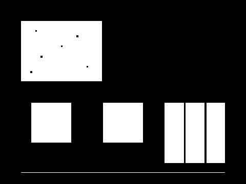
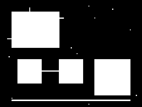
Applying each once to the test scene with a 3×3 rectangular structuring element gives Figure 8.2. After erosion the foreground drops from 47426 px to 44233 px, and the blob count plummets from 16 to 7: all 10 noise dots vanish, the burrs are stripped clean, and the 2 px thin bridge is severed — the merged double blob splits in two. The cost is equally visible to the naked eye: every target has slimmed down by one ring, the pepper holes are enlarged, and the thin gaps grow wider. Dilation does the opposite: the foreground swells to 50603 px, the pepper holes are filled, the 1 px and 2 px thin gaps both close up, but every target has fattened by one ring, and the noise dots, far from disappearing, have grown.

Each operation solves only half of the problem, and each introduces a new one — the size changes. In measurement applications this is unacceptable: erode once, and the target’s area and contour positions are systematically biased small; dilate once, and they are biased large. How can we enjoy the benefits of “deleting noise / filling gaps” while getting the size back? The answer is to chain the two together.

8.2 Opening and Closing

Opening is defined as erosion followed by dilation:

\[ A \circ B = (A \ominus B) \oplus B, \]

while closing is dilation followed by erosion:

\[ A \bullet B = (A \oplus B) \ominus B. \]

The design idea behind both is the same: the first step “kills or spares” the target structures, and the second step approximately restores the survivors’ size. In opening, the erosion first deletes every small structure that cannot accommodate the structuring element — once gone, the subsequent dilation cannot bring them back; large targets, on the other hand, have merely slimmed by one ring, and the dilation puts that ring back. Closing acts dually on the background: the dilation first fills every small gap and hole that cannot accommodate the structuring element, and the erosion then shrinks the swollen targets back to their original shape.

Opening and closing are both idempotent: \((A \circ B) \circ B = A \circ B\), and likewise for closing. Doing it once and doing it a hundred times give exactly the same result — everything that should be deleted is deleted cleanly the first time, and the surviving structures already “accommodate the structuring element,” so further applications are just the identity. This is in stark contrast to the cumulative “the more you filter, the blurrier it gets” behavior of smoothing filters.

The experimental results are shown in Figure 8.3, and the numbers demonstrate “approximate size preservation” with great clarity. After the 3×3 opening the foreground is 47225 px, a mere 0.4% decrease relative to the original 47426 px; after the 3×3 closing it is 47801 px, a mere 0.8% increase — compared with the roughly ±6.7% change of erosion/dilation alone, opening and closing reduce the size deviation by an order of magnitude. And the decrease and increase are exact to the pixel: the 201 px deleted by the opening equals precisely the combined area of the 10 noise dots (22 px), the three burrs (59 px), and the thin bridge (120 px) — the rectangle bodies did not lose a single pixel; the 375 px added by the closing equals precisely the combined area of the two thin gaps (360 px) and all the pepper holes (15 px).

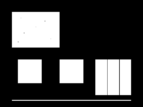
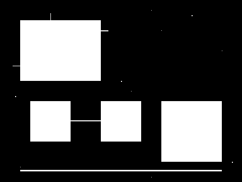
The blob counts further reveal the division of labor between the two. After opening, 7 blobs remain: the 10 noise dots are gone, the thin bridge is severed (the merged pair splits in two), and the burrs are removed clean — but the pepper holes inside the rectangle are still there. Opening does not fill holes: it only deletes small protruding structures in the foreground and is powerless against small holes in the background. After closing, 14 blobs remain: the 1 px and 2 px gaps are both sealed, the three severed pieces rejoin into one, and the pepper holes are filled — but not one of the 10 noise dots is gone. Closing removes neither burrs nor noise dots. This is duality made visible: opening repairs the “excess” of the foreground, closing repairs the “excess” of the background, and neither can substitute for the other. In real engineering the two are often chained — open first, then close: sweep away the noise before sealing the broken gaps. The counts for all operations in this chapter are summarized in Table 8.1.

Table 8.1: Effect of each morphological operation on the test scene’s foreground pixels and blob count

Operation	Foreground pixels	Relative to original	Blob count (8-connectivity)
Original scene	47426	—	16
Erosion 3×3	44233	−6.7%	7
Dilation 3×3	50603	+6.7%	—
Opening 3×3	47225	−0.4%	7
Closing 3×3	47801	+0.8%	14
Opening 5×5	46025	−3.0%	6

8.3 Choosing the Structuring Element Size

Opening and closing hand the decision of “what to delete, what to keep” entirely to the size of the structuring element — whatever cannot accommodate it dies, whatever can survives. So is a bigger structuring element always safer? Swap the opening’s structuring element from 3×3 to 5×5 and run again (Figure 8.4): the foreground drops to 46025 px and only 6 blobs remain. The one that went missing is not noise — it is the 3 px-thick thin strip. It accommodates a 3×3 structuring element but not a 5×5 one, so it was wiped out root and branch. If that “thin strip” were a lead wire or a genuine scratch on the product, the inspection system would have destroyed the evidence with its own hands at the preprocessing stage.

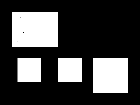
Figure 8.4: 5×5 opening: the noise is removed just as cleanly, but the 3 px thin strip is wiped out in its entirety as well (blob count 16→6) — once the structuring element is larger than the structures to be kept, deletion no longer distinguishes noise from target.

This yields the most important engineering rule of the chapter: the structuring element must be larger than the noise to be deleted and smaller than the smallest structure to be kept. In this example the largest noise is 2×2 and the smallest genuine structure is 3 px thick, so 3×3 lands exactly in the gap while 5×5 oversteps it. If the two bounds conflict — the noise grains are larger than the smallest target — then the single dimension of size can no longer separate them; do not force the structuring element, but switch to structuring elements of different shapes (an elongated structuring element for elongated targets) or leave the residual noise to downstream area-based screening.

This rule is isomorphic to the median-filter kernel-size rule of Chapter 6: the median kernel must be smaller than twice the width of the smallest structure to be preserved, or thin lines are wiped out together with the noise. This is no coincidence — opening and the median filter both belong to the family of nonlinear filters that “keep or discard by size ranking”; neither knows “defect” from “noise” — they only know size.

8.4 Grayscale Morphology and the Top-Hat

The min/max view mentioned in Section 8.1 lets morphology walk naturally out of the binary world: for grayscale images, grayscale erosion takes the minimum gray value within the structuring element’s neighborhood, and grayscale dilation takes the maximum. Grayscale opening (min then max) shaves off every bright peak “too narrow to accommodate the structuring element,” while leaving large-area background undulations almost untouched — in other words, grayscale opening is an operation that keeps only the background.

This immediately spawns an industrial power tool. The white top-hat transform is defined as the original image minus its grayscale opening:

\[ T_b(f) = f - (f \circ b). \]

\(f \circ b\) is “an estimate of the background with the small bright structures wiped out”; subtracting it from the original leaves exactly those small bright structures themselves — whether the background is flat, slanted, or curved, it is subtracted away clean. The top-hat is naturally immune to the background brightness level, which is exactly what shading correction in Chapter 4 tries to achieve: think of the top-hat as “small-target extraction with a built-in background estimate” — the background model needs no separate capture and no fitting; it is hidden inside the opening.

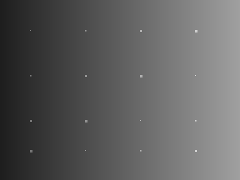
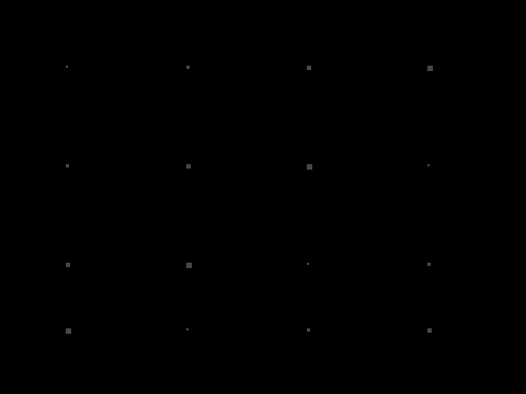
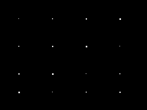
The experimental scene (Figure 8.5) is deliberately designed to defeat the global thresholding of Chapter 7: the background is a horizontal gradient from 30 to 160, on which 16 small bright spots (ranging from 2×2 to 5×5) are superimposed, each 70 gray levels brighter than its local background. The darkest spot, located on the left side of the image, peaks at only about 116, while the brightest background on the right is already 160 — the spots are darker than the background, so no global threshold capable of separating the two exists. After a white top-hat with an 11×11 structuring element (larger than the largest 5×5 spot), the gradient background is subtracted wholesale; binarizing at threshold 35 then extracts exactly 16 blobs totaling 216 px — in perfect agreement with the ground-truth area of the 16 spots (\(4\times(4+9+16+25)=216\)), not one pixel more, not one less. The top-hat’s structuring-element size rule is the same as in the previous section, but flipped: it must be larger than the targets to be extracted, so that the opening wipes them out of the background estimate and they appear in the difference.

8.5 SciVision Implementation

The morphology functionality of the SciVision SDK is provided by two classes, SciMorphStructure (structuring element) and SCIMV::SciSvMorphology (operations). The invocation consistent with this chapter’s experiments is as follows:

// Structuring element: CreateElement(rows, cols, anchorX, anchorY, shape, data)
SciMorphStructure se3, se11;
long rc = se3.CreateElement(3, 3, 1, 1, SCI_MS_RECT);    // 3×3 rectangle, anchor (1,1) centered
if (rc) { /* return codes must be checked */ }
rc = se11.CreateElement(11, 11, 5, 5, SCI_MS_RECT);      // 11×11 for the top-hat

SciROI roi;
SciPoint tl(0, 0), br(W, H);   // GenRect1's bottom-right is an exclusive endpoint: pass (W,H) for the full image
roi.GenRect1(tl, br);          // takes non-const references, so named variables are required

SCIMV::SciSvMorphology m;
SciImage dErode, dOpen, dTop;
rc = m.Erode(src, roi, se3, 1, &dErode);     // erosion, iteration = 1
rc = m.Open (src, roi, se3, 1, &dOpen);      // opening
rc = m.TopHat(gsrc, roi, se11, 1, &dTop);    // white top-hat

The first two parameters of CreateElement are the structuring element’s row and column counts; anchorX/anchorY specify the anchor position (conventionally the center, e.g., (1,1) for 3×3 and (5,5) for 11×11); shape set to SCI_MS_RECT means a solid rectangle, and the final int* data parameter is used only for custom shapes — it can be omitted for rectangular kernels. The five interfaces Erode/Dilate/Open/Close/TopHat share the same signature: input image, ROI, structuring element, iteration count, and output pointer. The iteration parameter is the number of times the operation is repeated — for rectangular structuring elements, \(n\) iterations of a 3×3 erosion are equivalent to a single \((2n+1)\times(2n+1)\) erosion, so small-kernel iteration can substitute for a large kernel; but for opening and closing, idempotence means iteration greater than 1 may give the same result as 1, so it is normally fixed at 1.

One pitfall that must be reported honestly: the bottom-right corner of SciROI::GenRect1 is an exclusive endpoint (the same semantics were already recorded in the SciVision section of Chapter 7). If you follow the “coordinate of the last pixel” intuition and pass \((W-1,H-1)\), the last row and last column are excluded from the ROI and left unprocessed — the morphology output is identically 0 along that border band, the top-hat difference \(f - 0\) degenerates to the original gray value, and the brighter side of the gradient background is left with a strip of high response strong enough to punch through the threshold. This artifact is easily misread as an SDK defect of “not processing the outermost row/column”; in fact, once you pass \((W,H)\) (or simply use an undefined ROI), the SDK processes the complete image and the artifact vanishes. All experiments in this chapter were run with a full-image ROI of \((W,H)\).

Industry Case: Opening to the Rescue in Solder-Joint Inspection

At a PCB solder-joint inspection station, solder-paste splatter left large numbers of 1–3 px small bright grains on the board surface; after thresholding they all became foreground, and the blob count overstated the true number of solder joints several times over. Inserting a single 3×3 opening between segmentation and counting removed the splatter grains clean and the count returned to normal — a textbook application of opening. Three months later an engineer changed the structuring element to 7×7 on the grounds that it was “safer”: the splatter was indeed removed even more thoroughly, but the line immediately began missing joints — the smallest-specification solder joint on that product was only 6 px in diameter, could not accommodate a 7×7 structuring element, and was wiped out together with the splatter. The post-mortem conclusion was written into the department standard: the upper bound on the structuring element size must be derived backward from the minimum solder-joint size in the process documentation, not forward from “how cleanly the noise is removed”; leaving residual splatter to downstream area-based screening is far safer than enlarging the structuring element.

8.6 Summary

Morphology is the repair step between thresholding and blob analysis: erosion deletes pixels by the rule “the structuring element must fit entirely inside the foreground,” dilation adds pixels by the rule “set the pixel whenever the structuring element touches the foreground”; the two are duals, equivalent to neighborhood min/max filters, but used alone each systematically changes target size (about ±6.7% in this chapter’s experiments).
Opening = erode then dilate: removes noise dots, burrs, and thin bridges but does not fill holes; closing = dilate then erode: seals thin gaps and fills small holes but does not remove noise dots. Both keep the size deviation within ±1% (47426 → 47225 / 47801), and both are idempotent — once is enough.
The structuring-element size rule: larger than the noise to delete, smaller than the structures to keep (3×3 spares the 3 px thin strip; 5×5 wipes it out). This is isomorphic to the median-filter kernel-size rule — nonlinear filters only know size, not semantics.
The white top-hat \(f-(f\circ b)\) is small-bright-target extraction with a built-in background estimate, immune to illumination gradients: in a gradient scene where any global threshold must fail, a single fixed threshold after the top-hat extracts all 16 bright spots exactly, with 216 px matching the ground truth. The structuring element must be larger than the targets to extract.
Engineering reminder: the bottom-right corner of GenRect1 is an exclusive endpoint — passing \((W-1,H-1)\) excludes the last row/column from processing, and the top-hat degenerates to the original gray value along that border band; a full-image ROI must pass \((W,H)\).

The theoretical origin of mathematical morphology is Serra’s foundational monograph (Serra 1982), while Soille’s book systematically covers grayscale morphology and its applications (Soille 2004); for a unified review of binary and grayscale morphological operators, see the classic paper by Haralick, Sternberg, and Zhuang (Haralick, Sternberg, and Zhuang 1987). For the complete theoretical edifice of morphology (advanced topics such as the hit-or-miss transform, geodesic reconstruction, and the watershed), see the book by Steger et al. (Steger, Ulrich, and Wiedemann 2018).