9 Gray-Level Transforms and Histograms

One of the most common complaints heard on a production line is “the image is too gray”: the target and the background differ in gray level, yet to the eye they blur into one indistinct mass. Faced with such an image, the first instinct is to adjust the contrast — and “adjusting contrast” corresponds at the algorithmic level to the simplest class of image operations there is: the point operation. A point operation is defined by the property that the output gray level of a pixel depends only on the input gray level at the same position, i.e. \(s = T(r)\), with no neighborhood involved whatsoever. This stands in sharp contrast to the spatial filtering of Chapter 6 — a filter looks at a neighborhood, a point operation looks only at itself. For an 8-bit image, every point operation reduces to one and the same implementation form: the lookup table (LUT) — precompute all 256 output values \(T(0)\) through \(T(255)\), store them in a table, and at processing time each pixel costs exactly one table lookup. The contrast stretching, gamma correction, and histogram equalization of this chapter are, at bottom, all answers to a single question: how should those 256 table entries be filled in.

The engineering value of the LUT is that it unifies “an arbitrarily complex gray-level mapping” into one \(O(1)\) table lookup per pixel: first evaluate \(T(r)\) once for each of the 256 gray levels, then sweep the image once. Whether \(T\) is piecewise linear, a power function, or a CDF, the running cost is exactly the same.

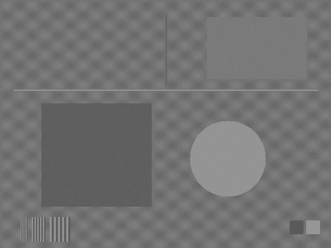
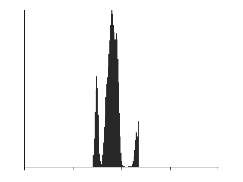
Throughout this chapter we use one synthetic low-contrast scene (480×360) for all experiments: on a sinusoidal-texture background sit a flat plate of constant gray level, a dark rectangle, a bright circle, two thin 2 px lines, and a set of resolution stripes, plus two anchor blocks that pin the gray-level range precisely to 90 and 150 — the gray values of the entire image occupy only \([90,150]\), using less than a quarter of the 8-bit dynamic range. Figure 9.1 shows the scene and its histogram.

9.1 The Histogram: The Image’s Gray-Level Ledger

The histogram is a statistic of the image’s gray-level distribution: the count \(h(k)\) of the \(k\)-th bin equals the number of pixels whose gray value is \(k\). Dividing the counts by the total number of pixels \(N\) gives the normalized histogram \(p(k)=h(k)/N\) — which is precisely a concrete instance of the “empirical distribution” of Chapter 2: if “the gray value of a randomly drawn pixel” is viewed as a random variable, \(p(k)\) is the empirical estimate of that variable’s distribution. The histogram discards all spatial information (shuffle the image’s pixels and the histogram is unchanged), yet it condenses everything about exposure and contrast into a single curve.

Reading a histogram is a basic skill. Counts piled up against 0 at the left end mean underexposure (the shadows are clipped); piled up against 255 at the right end, overexposure (the highlights are saturated, and no software can ever recover the clipped information — that has to be fixed back at the illumination design of Chapter 4); whereas counts squeezed into a narrow mid-range band, as in Figure 9.1 (b), are the signature of low contrast: the exposure is fine, but the scene itself has little reflectance contrast or lens flare has lifted the shadows. For this chapter’s scene, the SDK statistics give: mean 114.78, gray-level standard deviation 12.55, range exactly \([90,150]\). A standard deviation of only 12.55 — for an 8-bit image, that is the quantitative way of saying “everything is one gray mush.”

9.2 Linear Stretching

Since the gray values occupy only \([r_{\min}, r_{\max}]=[90,150]\), the most direct fix is to stretch this interval linearly to fill \([0,255]\):

\[ s = (r - r_{\min}) \cdot \frac{255}{r_{\max} - r_{\min}}. \]

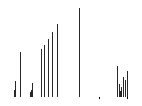
This is a straight line of slope \(255/60 = 4.25\) — every pixel’s gray value (noise included) is amplified by a factor of 4.25. Figure 9.2 shows the stretched result: the texture, the thin lines, and the stripe group are all clearly distinguishable; statistically the mean is 105.30, the standard deviation leaps from 12.55 to 53.34, and the range fills \([0,255]\).

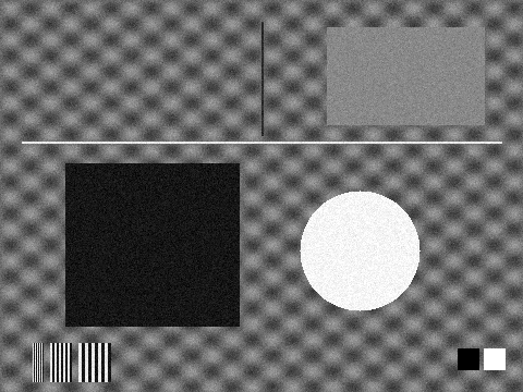
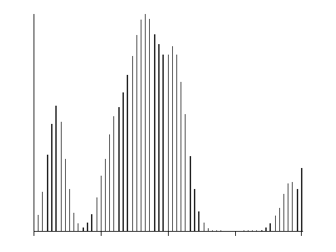
The histogram after stretching (Figure 9.2 (b)) exhibits the textbook comb artifact: the input contains only 61 discrete gray levels, and an integer LUT maps them to at most 61 output levels within \([0,255]\) — the remaining nearly 200 bins are doomed to stay empty. Stretching creates no new information whatsoever; it merely spreads the existing 61 gray levels out along the axis, and the number of distinguishable gray levels does not increase by even one. This is also a useful diagnostic: when you see a comb-shaped histogram, you can be fairly confident the image has been digitally stretched.

In practice, stretching directly from the image’s global minimum and maximum is not robust — a single bad pixel can drag \(r_{\min}\) or \(r_{\max}\) to an extreme value and defeat the stretch. The standard engineering remedy is percentile-clipped stretching: discard the darkest and brightest \(p\%\) (e.g. 1%) of pixels before taking the interval endpoints, buying immunity to outliers at the cost of sacrificing a tiny fraction of pixels.

9.3 Gamma Correction

Linear stretching treats all gray levels alike; to selectively brighten the shadows or darken the highlights, a nonlinear mapping is needed. The most common one is the power-law gamma correction:

\[ s = 255 \cdot \left(\frac{r}{255}\right)^{\gamma}. \]

The intuition behind the curve is simple: for \(\gamma<1\) the curve bows upward — the slope in the shadows exceeds 1 (they are spread apart and brightened) while the slope in the highlights is below 1 (they are compressed); for \(\gamma>1\) it is the reverse — shadows compressed, highlights expanded. The endpoints \(0\mapsto 0\) and \(255\mapsto 255\) never move; only the allocation of the midtones changes. Probing the SDK’s convention with a 0–255 gray ramp: at \(\gamma=0.5\), \(64\to 128\), \(128\to 181\), \(192\to 221\) — the output is always greater than the input, consistent with the formula above (input normalized first, then raised to the power).

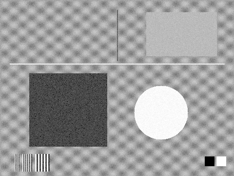
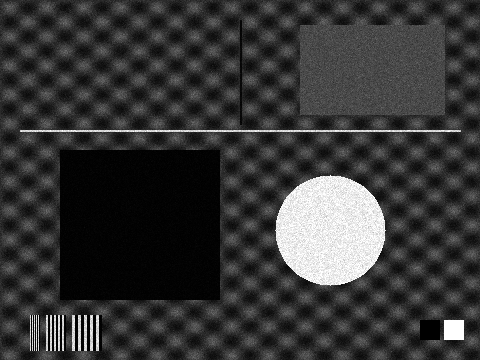
Measured on the stretched image (Figure 9.3): the interior of the dark rectangle (mean 21.4 after stretching) is lifted to 71.8 by \(\gamma=0.5\) and crushed to a mere 2.3 by \(\gamma=2.0\); the interior of the bright circle (245.6) rises only slightly to 250.0 under \(\gamma=0.5\) and dips slightly to 236.8 under \(\gamma=2.0\). The numbers confirm the shape of the curve: nearly all of gamma’s “muscle” is spent on the side far from the endpoints — \(\gamma<1\) moves the shadows dramatically while barely touching the highlights, and \(\gamma>1\) does the opposite.

The word “gamma” comes from the display chain: a traditional monitor’s luminance response is approximately \(V^{2.2}\), so consumer images (sRGB) are pre-encoded with the inverse \(\gamma\approx 1/2.2\) at storage time. Industrial cameras, by contrast, output linear gray values by default — pixel value proportional to luminous flux, which is exactly what measurement algorithms want. Introducing gamma into a measurement pipeline means destroying the linear photometric relationship and should be done only with great caution; its legitimate uses are display and human visual inspection.

9.4 Histogram Equalization

Stretching and gamma both require parameters to be chosen by hand; histogram equalization lets the image decide its own mapping — the goal is to make the output histogram as flat as possible. The derivation takes just one step: to “flatten” the distribution, densely populated gray ranges should be spread apart and sparse ones compressed, and the cumulative distribution function (CDF) has exactly this property built in. Define \(\mathrm{CDF}(r)=\sum_{k\le r} p(k)\) and take the mapping

\[ s = T(r) = 255 \cdot \mathrm{CDF}(r), \]

then \(T\) is monotonically nondecreasing (it never reverses the gray-level order), and its local slope is proportional to the histogram density \(p(r)\) at that point — where pixels crowd together, the slope is steepest and the values are pulled apart the most. Equalizing this chapter’s scene gives the result in Figure 9.4: the standard deviation rises further to 74.28 (mean 131.30), a contrast even beyond linear stretching.

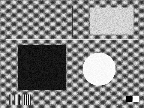
But look closely at the “flat plate” in the upper right of Figure 9.4 (a): in the original it was a constant gray level of 122 plus \(\sigma=2\) noise, and now it is covered in grain. Quantitatively measuring the standard deviation inside this plate yields the most important set of numbers in this chapter: 2.02 in the original, 8.46 after linear stretching (a factor of 4.19 — almost exactly the LUT’s constant gain of \(255/60\)), but 18.02 after equalization — an amplification of 8.93×, more than double that of linear stretching. The reason lies precisely in the slope of the CDF: the flat plate’s several thousand pixels are all crammed into two or three bins around 122, where \(p(r)\) is extremely high, so the local slope of \(T\) is at its steepest — equalization amplifies gray-level differences (noise included) most fiercely exactly where pixels are most densely packed, and flat regions are precisely where pixels pack most densely.

This settles equalization’s place in engineering: it is a tool for “showing images to people” — well suited to visual inspection, report figures, and manual-review interfaces; but it should be used with great caution in measurement and defect-detection pipelines. The automatic thresholding methods of Chapter 7 rest on the statistical premise that “foreground and background each have concentrated gray values,” and equalization systematically destroys exactly that premise: once the noise in flat regions has been amplified nearly 9-fold, a previously clean background sprouts a host of spurious responses that cross the threshold.

Equalization’s local gain \(T'(r) \propto p(r)\) also explains a seemingly paradoxical fact: its boost to genuine structural contrast and its amplification of flat-region noise come from one and the same mechanism — you cannot have the former without the latter. Adaptive variants (such as CLAHE’s clip limit) mitigate this conflict precisely by capping the slope at densely populated bins.

9.5 SciVision Implementation

This chapter’s experiments involve three classes: histogram statistics SciSvHistogram, stretching and equalization SciSvHistEqualize, and gamma SciSvBrightness.

SCIMV::SciSvHistogram histOp;
SciROI roi;                       // default-constructed = UNDEF ROI, which the SDK takes to mean the whole image
SciVarArray histData, histRange;
double avg, stdValue; int mn, mx, med, norm, total;
// lower=0, upper=255 statistics range; type=4 custom bin count; nBins=256, i.e. one bin per gray level
histOp.CaculateHist(img, roi, 0, 255, 4, 256, &histData, &histRange,
                    &avg, &stdValue, &mn, &mx, &med, &norm, &total);

SCIMV::SciSvHistEqualize eq;
SciImage stretched, equalized;
// method=1 clipped linear stretching; lowPct/highPct=0 means stretch [minGray,maxGray]=[90,150] fully onto [0,255]
eq.LineStretchHist(scene, roi, 1, 0.0, 0.0, 90, 150, &stretched);
// rangeValue=255 full-range equalization; minStrength=0 / maxStrength=255 is the default strength interval
eq.EqualizeHist(scene, roi, 255, 0, 255, &equalized);

SCIMV::SciSvBrightness bright;
SciImage dst;
bright.AdjustGamma(img, roi, 0.5f, &dst);   // s = 255*(r/255)^gamma

A single call to CaculateHist returns the histogram array together with a set of statistics, but there is one pitfall you must know about: the output parameter stdValue is the standard deviation of the 256 bin counts, not of the pixel gray values — for this chapter’s original image it returns 157.61, which already exceeds 127.5, the theoretical upper bound of an 8-bit gray-level standard deviation, so it is clearly not a gray-value statistic. The values 12.55/53.34/74.28 quoted in the text are all gray-level standard deviations computed from the histogram ourselves. LineStretchHist with method=0 (automatic stretching from the global min-max) was found to apply no transform at all to this image — a suspected SDK defect — so we use method=1 and specify [minGray, maxGray] explicitly. Also, do not construct the full-image ROI as GenRect1((0,0),(W-1,H-1)) — that rectangle is treated as a half-open interval, and the last row and column, 839 pixels in total, are excluded from the statistics; simply use a default-constructed UNDEF ROI to denote the whole image. One final detail: a pixel-by-pixel comparison of the SDK’s stretch against a hand-written LUT following the formula shows a maximum difference of just 1 (from truncation-versus-rounding differences in integer conversion), confirming that LineStretchHist is internally exactly a lookup-table point operation.

The complete runnable project is located at code/gray_transforms_histograms/, with fixed random seeds to ensure reproducibility.

Industry Case: Two Ways to Fix “the Image Is Too Dark”

A production line reported that its inspection images were dark and low in contrast. The software team’s first “fix” was histogram equalization — the picture instantly became crisp and good-looking. Two weeks later the defect false-alarm rate had doubled: the sensor noise in the flat background regions had been amplified several-fold by the equalization (the 2.02→18.02 of this chapter replayed on the factory floor), and swarms of noise pixels crossed the defect-decision threshold and were reported as phantom defects. The correct fix, established in the post-mortem, came in two steps. Step one: go back to the hardware chain — check the exposure time, the aperture, and the lens; bring the analog gain down; and obtain, at the source, an image with sufficient gray-level range and controlled noise (see Chapter 4 and Chapter 1). Step two: in software, apply only a parameter-controlled percentile-clipped linear stretch, and feed the post-stretch noise level back into the threshold tuning. The lesson fits in one sentence: looking good and measuring well are two different things — the high-contrast image the human eye likes is not necessarily the low-noise image the algorithm needs.

9.6 Summary

Point operation = lookup table. Any operation whose output depends only on the input gray value at the same position is a point operation; on 8-bit images every one of them can be implemented as a 256-entry LUT. Stretching, gamma, and equalization are merely three different strategies for filling that table.
The histogram is the empirical distribution of gray values: it throws away spatial information yet retains all the evidence about exposure and contrast — piled against the left end means underexposure, against the right end means overexposure (the information is unrecoverable), squeezed into a narrow mid-range band means low contrast.
Linear stretching creates no information: spreading 61 gray levels across 256 leaves the number of distinguishable levels unchanged and leaves comb-shaped gaps in the histogram; the endpoints should be clipped percentiles rather than the global min-max, to resist outliers.
Gamma correction redistributes the midtones nonlinearly: \(\gamma<1\) lifts the shadows and compresses the highlights, \(\gamma>1\) the reverse, with the endpoints fixed; industrial cameras output linear gray values by nature, so introducing gamma into a measurement pipeline demands caution.
Equalization fills the table from the CDF, with local gain proportional to histogram density — flat regions are where pixels are densest and where noise is amplified most fiercely (8.93× measured in this chapter, far beyond linear stretching’s 4.19×). It is an enhancement tool for human viewing; before letting it into a measurement/inspection pipeline, first assess the damage to the statistical premises of Chapter 7.

The standard treatment of gray-level transforms and histogram processing (including global histogram equalization) is the textbook by Gonzalez and Woods (Gonzalez and Woods 2018); to counter the very drawback of global equalization amplifying noise in flat regions, the adaptive histogram equalization and its clipped variant (the precursor of CLAHE) proposed by Pizer et al. is the classic remedy (Pizer et al. 1987). For a systematic treatment of gray-level transforms and histogram processing in industrial pipelines (including robust stretching and polynomial gray-level correction), see the book by Steger et al. (Steger, Ulrich, and Wiedemann 2018).