5 Camera Calibration
Up to this point, every result in this book has been expressed in pixels: the edge sits at column 312.46, the circle center is off by 0.8 pixels. But acceptance criteria on a production line are never written in pixels — drawings are dimensioned in millimeters, tolerances read ±0.02 mm, and the robot arm needs positions in the workpiece coordinate frame. Camera calibration is the bridge from “pixels” to “millimeters”: it measures the camera’s own imaging parameters, after which every pixel coordinate can be converted into a physically meaningful geometric quantity. Without calibration, all the measurements of Chapter 21 are merely a game of pixels; and if the calibration is done poorly, even the cleverest algorithm will report lens distortion as workpiece deformation.
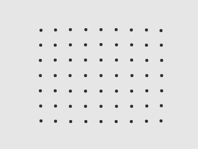
This chapter answers three questions: what the imaging process of a real camera looks like mathematically (pinhole model + intrinsics + distortion); how to recover these parameters from a few images of a calibration target (the principle and workflow of Zhang’s method); and the step most easily neglected — how to verify that a calibration result can be trusted. Running through the first four sections is a “ground truth known” synthetic experiment: we build a virtual camera by hand and let it photograph a calibration target (Figure 5.1), then use SciVision to calibrate the parameters back and reconcile them against the truth, item by item — because a real camera’s intrinsics are nowhere to look up, only a synthetic ground truth allows item-by-item verification. The final section then switches to a real calibration board, grounding the opening “pixels-to-millimeters” bridge in a nine-point coordinate calibration on an actually-photographed dot target (Section 5.5).
5.1 The Complete Imaging Model
Chapter 3 gave the intuition of the pinhole model: a scene point, the optical center, and the image point lie on one line. Written in matrix form with the homogeneous coordinates of Chapter 2, the projection of a world point \((X,Y,Z)\) onto a pixel \((u,v)\) is
\[ s\begin{bmatrix}u\\ v\\ 1\end{bmatrix} =\underbrace{\begin{bmatrix}f_x & 0 & c_x\\ 0 & f_y & c_y\\ 0 & 0 & 1\end{bmatrix}}_{K} \begin{bmatrix}R & \mathbf t\end{bmatrix} \begin{bmatrix}X\\ Y\\ Z\\ 1\end{bmatrix}. \]
The \([R\ \,\mathbf t]\) on the right is the extrinsics — the camera’s pose relative to the world coordinate frame, which changes with every new camera placement; the \(K\) on the left is the intrinsics matrix, determined solely by the camera and lens themselves. \(f_x,f_y\) are focal lengths in pixel units (the physical focal length divided by the pixel pitch in the horizontal and vertical directions; with square pixels the two are equal); \((c_x,c_y)\) is the principal point, i.e. where the optical axis pierces the sensor, which due to assembly tolerances is usually not at the exact image center. The meaning of the intrinsics can be summed up in one sentence: \(f_x\) scales “normalized coordinates” (the tangent of the horizontal viewing angle) up into pixels, and \(c_x\) then shifts the origin to the image’s top-left corner — once \(K\) is known, pixel coordinates and ray directions can be converted back and forth.
A real lens still lacks one final puzzle piece: distortion. The magnification of a lens assembly varies with field angle, causing image points to deviate radially from the position the pinhole model predicts. The Brown radial model describes this deviation with a polynomial in normalized coordinates:
\[ x_d = x_u\,(1+k_1 r^2 + k_2 r^4),\qquad y_d = y_u\,(1+k_1 r^2 + k_2 r^4),\qquad r^2=x_u^2+y_u^2, \]
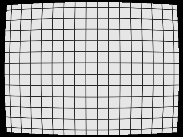
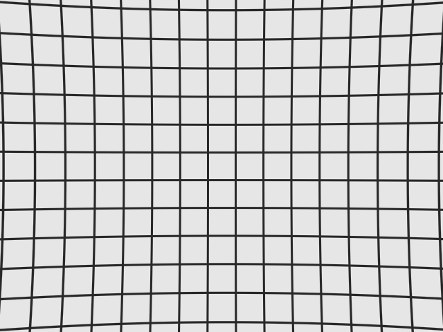
where \((x_u,y_u)\) are the ideal (undistorted) normalized coordinates and \((x_d,y_d)\) is the actual imaged position. With \(k_1<0\) the magnification decreases toward the field edge and straight lines bow outward into a barrel shape; with \(k_1>0\) they cave inward into a pincushion shape. Figure 5.2 visualizes both with a regular grid image: after applying this chapter’s virtual camera distortion \(k_1=-0.18,\ k_2=0.05\), the “straight lines” near the edges are visibly bent. The bending can be quantified — taking 61 analytically sampled points on one horizontal grid line at the top of the image and running an orthogonal regression, the distorted points deviate from the fitted line by at most 4.678 px, with an RMS of 2.249 px. Compared with the 0.1 px-level subpixel localization accuracy of Chapter 14, this is a systematic error one and a half orders of magnitude larger: without distortion correction, subpixel accuracy is meaningless.

The full Brown model also includes tangential distortion terms \(p_1,p_2\), which arise when the lens assembly and the sensor are not strictly parallel. Machine vision lenses are assembled to fairly tight tolerances, so the tangential component is typically more than an order of magnitude smaller than the radial one; this chapter’s experiments therefore keep only the first two radial orders \(k_1,k_2\) — which is also the default configuration of most industrial calibrations. SciVision’s calibration output likewise reserves slots for \(p_1,p_2\) (see Section 5.6).
5.2 The Principle of Calibration
The unknowns to be estimated are \(f_x,f_y,c_x,c_y\) and \(k_1,k_2\), plus a separate set of extrinsics for each image. The direct idea would be to photograph a known three-dimensional structure and solve backward, but 3D calibration objects are expensive to manufacture. Zhang’s method (Zhang 2000) cracked the problem using nothing but a planar target, and it remains the mainstream of industrial calibration to this day. Its reasoning proceeds in three steps.
Step one: each pose yields a homography. Points on the planar target satisfy \(Z=0\); substituting into the projection equation leaves only three columns of \([R\ \,\mathbf t]\), and the mapping from target plane to image degenerates into a 3×3 homography matrix \(H = K\,[\mathbf r_1\ \mathbf r_2\ \mathbf t]\) (up to scale). Each image’s own \(H\) can be solved from its point correspondences.
Step two: combine multiple poses to solve for initial intrinsics. \(\mathbf r_1,\mathbf r_2\) are columns of a rotation matrix and must be orthonormal — this imposes two constraints on \(K\) per homography \(H\). The intrinsics have 4 unknowns, so 3 distinct target poses already suffice for a closed-form solution; the more poses, the more stable the least-squares solution.
Step three: nonlinear refinement. The closed-form solution ignores distortion and serves only as an initial value. The final result comes from a nonlinear optimization: put the distortion coefficients and all the per-pose extrinsics into the parameter vector together, and minimize the reprojection error — the difference between each measured point position and the world point projected back into the image under the current parameters:
\[ \text{RMSE}=\sqrt{\frac{1}{N}\sum_{i=1}^{M}\sum_{j=1}^{N_i}\bigl\|\mathbf m_{ij}-\hat{\mathbf m}(K,k_1,k_2,R_i,\mathbf t_i,\mathbf M_j)\bigr\|^2}, \]
where \(\mathbf m_{ij}\) is the measured pixel coordinate of target point \(j\) in image \(i\), \(\hat{\mathbf m}(\cdot)\) is the prediction of the complete imaging model (distortion included), and \(N\) is the total point count. This quantity is also the primary indicator of calibration quality: it directly answers “to what extent does this parameter set explain the imaging process”.
Why must the calibration target be tilted at multiple angles? Imagine the target always facing the camera squarely: pull the camera twice as far away and double the focal length, and the resulting image is exactly the same — a fronto-parallel pose cannot distinguish \(f\) from the distance \(Z\); there is no information along the focal-length direction. A tilted pose breaks this degeneracy: the amount of perspective foreshortening between the near and far ends of the target is determined jointly by \(f\) and the tilt angle, and only then does the focal length become observable. This is the plainest example of the observability intuition: whether a parameter can be calibrated accurately depends on whether the data contains information about it, not on how good the optimizer is.
5.3 A Gold-Standard Experiment: Synthetic Calibration with Known Ground Truth
Real calibration suffers from a fundamental embarrassment: you never know the ground truth. The calibration reports \(f_x=1226.3\) — how far is that from the true focal length? Nobody can answer: a camera’s “true intrinsics” are simply nowhere to look up. The gold standard for validating a calibration algorithm is therefore a synthetic experiment: build a virtual camera with known parameters by hand, let it “photograph” the calibration target, feed the calibration algorithm as a black box, and reconcile its output against the truth item by item. This device validates not only the algorithm but also whether your understanding of the interface is correct — both engineering findings of Section 5.6 in this chapter were caught exactly this way.
The virtual camera’s ground truth is \(f_x=f_y=600\) (a horizontal field of view of about 56° at 640×480 resolution), \(c_x=326,\ c_y=243\) (the principal point deliberately offset from the image center), and \(k_1=-0.18,\ k_2=0.05\) (moderate barrel distortion). The calibration target is a 9×7 circle grid with 10 mm spacing, placed in 4 poses: fronto-parallel, pitched 20° about the X axis, yawed −20° about the Y axis, and a compound attitude (−15°/15°/10°). Gaussian noise with a standard deviation of 0.1 px is added to every projected point (with a fixed random seed for reproducibility), simulating the accuracy of real circle-center extraction. The 4×63=252 point pairs are fed to SciVision’s CameraCalibrate, with the following result:
| Parameter | Ground truth | Calibrated | Error |
|---|---|---|---|
| \(f_x\) | 600.0000 | 598.5707 | \(-1.4293\) |
| \(f_y\) | 600.0000 | 598.5468 | \(-1.4532\) |
| \(c_x\) | 326.0000 | 325.5661 | \(-0.4339\) |
| \(c_y\) | 243.0000 | 243.2207 | \(+0.2207\) |
| \(k_1\) | \(-0.1800\) | \(-0.1832\) | \(-0.0032\) |
| \(k_2\) | \(0.0500\) | \(0.0663\) | \(+0.0163\) |
Read the table line by line. The focal-length error is about 1.43 px, a relative error of 0.24% — ample for the vast majority of measurement applications; the principal-point error is under half a pixel. The reprojection RMSE is 0.1384 px, while the theoretical floor set by the point-extraction noise is \(\sqrt2\times0.1\approx0.1414\) px: the fitting residual has settled right onto the noise level, meaning the model has squeezed dry every bit of systematic information in the data — what remains is purely the random noise we injected ourselves.
Why is the noise floor \(\sqrt2\,\sigma\)? Reprojection error measures the magnitude of a two-dimensional residual vector; the \(u\) and \(v\) directions each contribute a variance of \(\sigma^2\), so the root mean square of the magnitude is \(\sqrt{2}\,\sigma\). That the RMSE comes in slightly below this value (0.1384 < 0.1414) is no surprise: the model has dozens of free parameters and absorbs a small share of the random noise along the way — a normal symptom of “fitting down to the noise level”. A result significantly below the noise floor, on the other hand, should raise overfitting alarms.
The only unflattering entry is \(k_2\): an error of 0.0163, off by 33% relative to the truth. This is not a failure of the algorithm but a limitation of the data — \(k_2\) multiplies \(r^4\), so only points at the extreme edge of the field of view get a say in it, and in this experiment the target’s projections never reached the corners of the frame. \(k_2\) sits in a weakly observable state: many combinations of \((k_1,k_2)\) are nearly equivalent over the range of \(r\) the data covers. Note that the reprojection RMSE did not suffer at all — within the region the data covers, this slightly-off parameter set and the ground truth make indistinguishable predictions. The pedagogical value of this exceeds the experiment itself: a parameter’s observability is determined by target coverage and tilt diversity — to calibrate \(k_2\) accurately, you must spread the target points into all four image corners. For the same reason, a calibration should be judged by its reprojection RMSE and the consistency of repeated recalibrations, not by trusting the parameter values themselves — in a real calibration you have no truth table to check against, and the parameters are free to drift along weakly observable directions.
5.4 Distortion Correction
With the parameters in hand, the next step is to remove the distortion from the image. The correct way to rectify an image is inverse mapping: for every pixel \((u,v)\) of the output (undistorted) image, use the forward distortion model to compute its source location \(F(u,v)\) in the original distorted image, then fetch the gray value by the bilinear interpolation introduced in Chapter 2. The direction must not be reversed — if input pixels were “scattered” forward into the output, their landing points would not sit on the integer grid and the output image would be left with holes. Inverse mapping guarantees that every output pixel is assigned exactly once, at the cost of one model evaluation plus one interpolation per pixel — which can perfectly well be precomputed into a lookup table.
We first validate the implementation with the pure model: applying a hand-written inverse-mapping + bilinear-interpolation correction to the barrel-distorted grid image, the orthogonal deviation of the top grid line drops from max 4.678 px to 0.000000 px (analytic sample points, no noise — zero to machine precision), proving that the inverse mapping and the interpolation are implemented strictly correctly. Figure 5.3 (a) is the corrected image, with the bent grid lines pulled straight again.
SciVision takes the engineering route. Calling the single-plane distortion calibration DistortionCalibrate on the 63 point pairs of the fronto-parallel pose returns Rms = 0.1493; the calibration matrix it outputs then serves two purposes. The first is point correction: using PointProject to transform distorted pixel coordinates into corrected pixel coordinates, the collinearity deviation of the 9 points in the target’s top row drops from 1.635 px before correction to 0.121 px — already close to the 0.1 px point-extraction noise level, with the systematic bending of the distortion essentially rooted out; fitting an affine transform from all 63 corrected points to the world grid leaves a residual RMSE of only 0.0329 mm and a maximum of 0.0782 mm, showing that the corrected image plane differs from the target plane by nothing more than a linear transform — from here on, pixels can be converted to millimeters by simple scaling. The second is image correction: DistortionCorrection directly outputs the undistorted image (Figure 5.3 (b)), visually consistent with the hand-written implementation’s result.
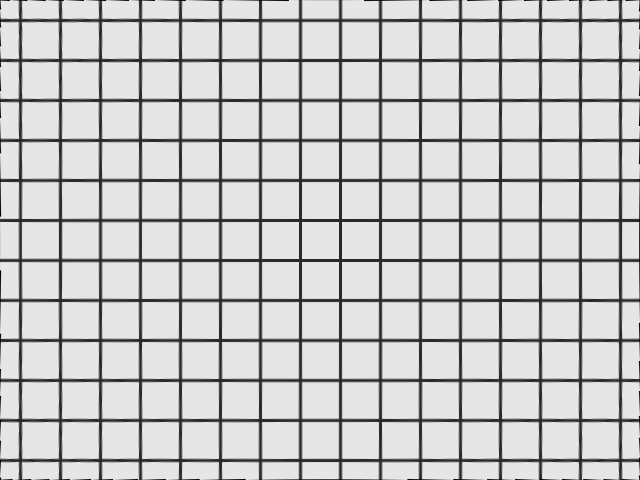

DistortionCalibrate result, with consistent output. The slight nibbling at the edges comes from the distorted image having no data beyond its borders.
5.5 A Real Calibration Board: Nine-Point Coordinate Calibration
The previous four sections used a virtual camera with known ground truth for intrinsic and distortion calibration — deliberately so: a real camera’s intrinsics are nowhere to look up, and only a synthetic ground truth allows item-by-item reconciliation (Section 5.3). But the chapter’s opening “pixels-to-millimeters” bridge has another, more direct realization that can be run end-to-end on a real calibration board — nine-point coordinate calibration. It does not estimate intrinsics; instead it uses a handful of known points on a planar target to fit the planar transform from “pixel coordinates” to “the target coordinate frame”, the form of calibration most commonly used in robot hand-eye alignment (SDK manual 4.2).
The sample image of this section is taken from the “nine-point calibration” example solution bundled with Smart3: a 3×3 dark-dot target on a \(1571\times1053\) grayscale image (Figure 5.4). The workflow has two steps. Extraction: we first try the SDK’s circle-board auto-detection FindImageCorners(gridType=1), but on such a sparse target of only 9 points it returns 122101001 (detection failure) — auto-detection is designed for dense checkerboard/circle arrays and degrades when points are too few; so we switch to deterministic connected-component centroids of the dark blobs, stably obtaining 9 circle centers with an average grid spacing of 236.2 px (rows 236.19, columns 236.23, indicating the target is nearly fronto-parallel with virtually no perspective). Calibration: feeding the 9 pixel centroids together with the target’s unit-grid coordinates \((-1,1)\dots(1,-1)\) (each cell is 1 world unit) to PointCalibrate yields the \(3\times3\) planar calibration matrix
\[ M=\begin{bmatrix}0.004233 & \approx\!0 & -3.0255\\[2pt] \approx\!0 & -0.004234 & 2.3963\\[2pt] 0 & 0 & 1\end{bmatrix}, \]
with pixel scales \(s_x=0.0042332,\ s_y=0.0042338\) world units per pixel (i.e. 236.2 px corresponds to 1 grid cell). Projecting the 9 points back to the target frame through \(M\), the fitting residual RMS is only 0.000106 world units (about 0.025 px), with a maximum point deviation of 0.000147 world units (about 0.035 px). This target is a software-rendered ideal dot array with no lens distortion, so a residual hugging the subpixel extraction accuracy is to be expected — its value lies in demonstrating the complete “pixels-to-coordinate-frame” closed loop on a real image.
More convincing is the cross-validation: the example solution ships with the calibration result the SDK’s graphical interface originally computed (calib_data.xml), whose matrix is \(a_{11}=0.004233,\ a_{22}=-0.004236,\ t_x=-3.027629,\ t_y=2.398271\) with scales \((0.0042328,0.00423579)\). Extracting points and calibrating independently in code, our linear coefficients and scales agree with these to the \(10^{-6}\) level, with the translation terms differing by about 0.002 world units due to the different extraction method (the interface rounds circle centers to the half-pixel) — our hand-written pipeline reproduced the result of the commercial interface, another way of grounding interface understanding in practice.
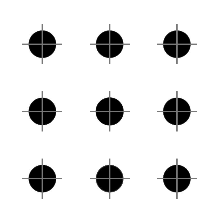
CalibImage/0.bmp). Gray crosses mark the 9 circle centers from hand-written centroid extraction; these 9 points fit the planar transform from pixels to the target coordinate frame via PointCalibrate, reproducing the SDK interface’s calibration result bundled with the example.
Why keep intrinsic/distortion calibration synthetic yet use a real board for coordinate calibration? The two are accepted in fundamentally different ways: the gold standard for intrinsic calibration is reconciliation against ground truth, which is unknowable for a real camera and hence must be synthetic (Section 5.3); nine-point coordinate calibration produces merely a “pixels-to-coordinate-frame” planar transform, whose quality is accepted via the fitting residual and reproducing a known solution, independent of any camera ground truth — so it can, and should, be run on a real target. The chapter thus splits in two: observability and accuracy analysis on the synthetic side, point extraction and coordinate calibration on real images on the real side.
5.6 SciVision Implementation
Multi-pose intrinsic calibration is performed by SCIMV::SciSvCalibration::CameraCalibrate, corresponding to the Zhang workflow of Section 5.2. The point correspondences of all poses are concatenated in order into two arrays, and an index array declares the point count of each view:
SCIMV::SciSvCalibration calib;
SciPointArray allImg, allObj;   // image/world points of the 4 poses, concatenated in order
SciVarArray ptsIndex;           // point count per pose (four 63s in this example)
for (int p = 0; p < 4; ++p) {
    for (size_t k = 0; k < wX.size(); ++k) {
        SciPoint ip(imU[p][k], imV[p][k]), op(wX[k], wY[k]);
        allImg.Append(ip); allObj.Append(op);
    }
    SciVar n((long)wX.size());
    ptsIndex.Append(n);
}
SciMatrix camMat;
double rmsC = -1;
long rc = calib.CameraCalibrate(allObj, allImg, ptsIndex,
                                /*W*/ 640, /*H*/ 480, &camMat, &rmsC);
allObj holds the target-plane coordinates (in mm; the planar target has \(Z=0\), so only 2D points are filled in), allImg the corresponding pixel coordinates; ptsIndex slices the flat arrays back into individual views, the image width and height are used for the intrinsics’ initial values, and the outputs are the parameter matrix camMat and the reprojection RMSE. Every number in Table 5.1 comes from this single call.
In use, this interface exposed two documentation problems, recorded here verbatim — they are exactly the situations engineers genuinely run into when integrating a commercial SDK. First, the element layout of the cameraParam matrix is not documented in the header. We reverse-engineered the actual layout from the synthetic experiment’s ground truth: row 0 is \([\,\_,\ f_x,\ c_x,\ f_y,\ c_y\,]\) and row 1 is \([\,k_1,\ k_2,\ p_1,\ p_2,\ \_\,]\) — without a truth table to check against, reading \(f_y\) and \(c_x\) swapped would not necessarily be noticed right away. Second, the behavior of PointProject does not match the header’s description. The documentation says it returns world coordinates, but when used with a distortion calibration matrix, what it actually returns is corrected pixel coordinates. Following the documentation at first, we subtracted its output directly from the world grid (in mm) and got an absurd “residual” of 427 mm; only after tracing the output’s units did we redesign the validation into the “fit an affine transform from corrected points to the world grid” scheme of Section 5.4. Both findings point to the same engineering habit: your understanding of an interface must be validated on data with known answers before it is used on a production line where the answers are unknown — which is the other dividend of the gold-standard experiment.
The real-board coordinate calibration of Section 5.5 uses another interface of the same module, PointCalibrate(imagePoint, worldPoint, type, …): it takes \(N\!\ge\!4\) pairs of pixel and target points and outputs a \(3\times3\) planar transform matrix, the pixel scales \(s_x,s_y\), and the fitting residual, with type=0/1/2 selecting planar / tilted / similarity (Helmert) calibration; when auto-detection fails, deterministic centroid extraction supplies the input side. The SciSvCalibration module also covers extended scenarios such as alignment/registration and hand–eye calibration (SDK manual 4.3): only by relating the camera coordinate frame to the motion platform’s coordinate frame can calibration results drive a robot arm. These belong, together with the 3D measurement of Chapter 30, to the downstream of the “calibration chain” and are not expanded here. The complete runnable project that generates all of this chapter’s experimental images and numbers lives in code/camera_calibration/.
Industry Case: Why Calibrations “Expire”
A structural-part measurement station passed acceptance smoothly at commissioning; three months later, a sampling check uncovered a systematic deviation of 0.03 mm. The diagnosis: heat buildup on the line expanded the lens barrel and shifted the focal plane, changing the effective focal length; vibration from the conveyor, meanwhile, rotated the camera bracket ever so slightly — intrinsics and extrinsics had both “expired”, with not a single line of the program changed. The countermeasure has two layers. One is periodic recalibration — redo the full calibration quarterly or at major maintenance milestones. The other, far cheaper, is a routine check: fix a reference standard of known dimensions in the field of view, measure it once per shift, and trigger recalibration only when a threshold is exceeded. Verification is far cheaper than calibration: one measurement, checked against one number, answers “can the calibration still be trusted”. In high-accuracy settings this check belongs on the equipment’s routine-check sheet — calibration parameters are not a software configuration but a physical measurement result that slowly drifts with temperature and vibration.
5.7 Summary
- The complete imaging model = pinhole + intrinsics + distortion: the intrinsics matrix converts ray directions into pixels, and the Brown radial model \(x_d=x_u(1+k_1r^2+k_2r^4)\) describes a real lens’s deviation from the pinhole. This chapter’s barrel distortion of \(k_1=-0.18\) bent straight lines by 4.678 px — without distortion correction, subpixel localization is meaningless.
- Zhang’s method runs “homography → closed-form initial value → nonlinear refinement”: each pose of the planar target contributes one homography and two intrinsic constraints; multiple poses jointly solve the initial value, and the final step minimizes the reprojection error. The target must be tilted at multiple angles — a fronto-parallel pose cannot distinguish focal length from distance.
- The synthetic gold-standard experiment is the gold standard for validating a calibration: only with known ground truth can you reconcile item by item. In this chapter’s experiment, the focal-length error was 0.24% and the reprojection RMSE of 0.1384 px hugged the \(\sqrt2\sigma=0.1414\) px noise floor — the information was squeezed dry; the outsized \(k_2\) error, meanwhile, exposed the weak observability caused by insufficient target coverage.
- Judge a calibration by reprojection RMSE and repeat consistency, not by the parameter values themselves: real calibrations have no ground truth to check against, and parameters will drift along weakly observable directions; image rectification uses inverse mapping + bilinear interpolation, and correction quality can be accepted quantitatively via geometric invariants such as collinearity (1.635 → 0.121 px).
- Interface understanding must pass the gold-standard experiment too: the parameter-matrix layout and the output units of
PointProjectwere both confirmed only by checking against ground truth — when documentation and implementation disagree, data with known answers is the only arbiter. - What runs end-to-end on a real board is nine-point coordinate calibration: with hand-written centroid extraction on Smart3’s actually-photographed 3×3 dot target (auto-detection fails on the sparse 9-point target),
PointCalibratefits the pixels-to-target planar transform with a residual of about 0.025 px, and its linear coefficients and scales reproduce the bundled SDK-interface solution to the \(10^{-6}\) level — intrinsic calibration is verified against synthetic ground truth, coordinate calibration against real data and reproduction of a known solution, each as appropriate.
For a systematic treatment of camera calibration (including richer distortion models, uncertainty analysis, and 3D calibration), read further in the book by Steger et al. (Steger, Ulrich, and Wiedemann 2018); Zhang’s original paper (Zhang 2000) is itself a very readable text. The modern treatment of distortion and intrinsics traces back to two classics: Brown (Brown 1971) gave, in close-range photogrammetry, the radial/tangential distortion model still in use today — this chapter’s \(k_1,k_2,p_1,p_2\) originate from it — while Tsai (Tsai 1987) proposed a two-stage technique for high-accuracy 3D metrology from a single target image, the industry mainstream before Zhang’s method. The extended scenario of relating the camera frame to a motion platform (SDK manual 4.3) is precisely hand-eye calibration, whose foundational algorithm is given by Tsai and Lenz (Tsai and Lenz 1989), solving the rigid transform between camera and end-effector from imaging at several known robot poses.