38 Point Cloud Preprocessing
Point a line-laser profilometer or a structured-light camera at a metal workpiece, press the capture button, and what you get back is never a clean, tidy 3D surface. The raw data carries three kinds of ailments mixed together: the height value jitters randomly at every sample point (the same origin as the noise in 2D images, except this time it is Z that jitters rather than gray value); scattered across the surface are patches of “black holes” — where the laser hits a steep wall, a deep bore, or a specular reflection and cannot be returned, those sample points get no height at all and become invalid pixels; and occasionally a few lonely “spikes” pop up, hundreds of microns above the true surface, the artifacts left by secondary reflections or anomalous matching. At the same time, a single range image easily contains hundreds of thousands to millions of points, and feeding it straight into registration or matching makes the computation explode in an instant. Noisy, full of holes, and far too dense — this is the raw stock that downstream measurement and inspection must confront. Point cloud preprocessing is the very first procedure before measurement. What it does corresponds one to one with the 2D image enhancement of Part III: denoising, gap filling, downsampling, segmentation — only the battlefield has moved from the gray image to the 3D surface. This chapter can be read as the 3D counterpart of 2D enhancement.
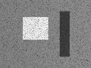
Figure 38.1 is the synthetic scene that runs through this entire chapter: a 320×240 = 76800-pixel range image, with a base height of 1000 μm and a gentle slope along the x direction, carrying a +400 μm boss and a −300 μm groove; onto it we have superimposed Gaussian height noise of σ = 5 μm, 5% invalid pixels (3858 invalid points in total, appearing as black spots in the figure), and then sprinkled 245 spikes (appearing as white spots). This single image gathers all three typical defects at once, and every section below starts from it.
38.1 Range Image vs. Point Cloud: Where to Do It
Three-dimensional data can be stored in two ways, and preprocessing can be performed on either, but the cost and reusability differ greatly.
The first is the range image, also called the depth map or 2.5D height map: it is essentially an image on a regular grid, where each pixel stores one height value (Z), and the horizontal and vertical coordinates are implied by the pixel position (Chapter 37). Its greatest benefit is “regularity” — all the 2D algorithms based on pixel neighborhoods in Part III, namely median filtering, Gaussian filtering, morphology, and threshold segmentation, can be transplanted almost unchanged, simply swapping “gray value” for “height.” The second is the unordered point cloud: a pile of discrete \((X,Y,Z)\) triplets that attach to no grid, able to faithfully express arbitrary topology (including overhangs, sidewalls, and multilayer structures that a range image cannot represent), but at the price of relying on a kd-tree for neighborhood queries, with every step running noticeably slower than on a regular grid.
Rule of thumb: for single-view, single-layer surfaces (which describes the vast majority of inline inspection), prefer processing on the range image — it lets you directly reuse the mature 2D algorithms, runs fast, and saves memory; only when the object has overhangs, requires multi-view stitching, or has topology too complex for a grid to express do you enter the world of unordered point clouds (Chapter 39).
For exactly this reason, most SDK 3D preprocessing operations are done on the range image, and this chapter’s main arena is set here too. But there is one pitfall that does not exist in the 2D world and must be made clear first: invalid pixels must not enter the computation as 0. In a range image, invalid points are often marked with a count of 0 (or some sentinel value), meaning “there is no data here,” not “the height here is 0.” If a filter treats this as a height value of 0 and folds it into an average, then the true height next to a hole gets dragged sharply downward by this false 0, and denoising ends up manufacturing a fake trough. Therefore every step of 3D filtering and morphology must be NaN-aware: only valid neighbors are counted, and invalid points neither contribute nor get contaminated. Every hand-written operator in this chapter obeys this rule, and we will see its effect again and again below.
38.2 3D Filtering
Denoising is the first step of preprocessing, and the idea is entirely consistent with Chapter 6: on the height map, take a neighborhood around each point and perform an appropriate “averaging” to suppress the random jitter. We let two classic filters compete on the range image — a 3×3 median filter and a 3×3 Gaussian filter, both implemented as NaN-aware versions: if the center is invalid it stays invalid; if the center is valid it takes the median of only the valid heights in the neighborhood (median filter) or their weighted average (Gaussian filter).
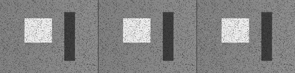
To measure the denoising effect, we look at the root-mean-square (RMS, in μm) of the flat base subregion’s height relative to the ground-truth plane. The results are as follows: the raw data has an RMS as high as 32.09 μm — note that this number is far larger than the 5 μm noise standard deviation, because it is heavily polluted by the 245 spikes. The median filter pushes the RMS down to 2.28 μm, the Gaussian filter only to 12.08 μm, while median-then-Gaussian (median to remove spikes, Gaussian to smooth random noise) achieves 1.61 μm, the best of the field.
The root of the gap lies in the spikes. The lesson from Chapter 6 — the median removes outliers, the Gaussian smears them — replays unchanged here in 3D. Counting the residual spikes (valid points with |measured height − ground truth| > 200 μm): 245 originally, only 5 remain after the median filter, while 14 still remain after the Gaussian filter. The median filter treats each spike as a local outlier; after sorting it gets pushed to the tail of the list, never gets a turn to be the output, and is thus cleanly eliminated. The Gaussian filter, however, spreads the spike’s few-hundred-micron height across its surrounding neighbors, and the result is not the elimination of the spike but smearing it into a shorter, fatter “bump” — the spike’s energy has not vanished, it has merely been painted out. Figure 38.2 places the three side by side, and the eye can plainly see that the white spikes in the raw image have completely disappeared in the median result, but have turned into patches of pale halos in the Gaussian result.
This section uses isotropic Gaussian/median filters. If you want both to suppress noise and to preserve the steep walls of the boss and groove, you can switch to an edge-preserving 3D filter — the bilateral filter or the guided filter — which introduces the “only participate in the average if the heights are close” criterion into the weighting, with a mechanism stemming from the same lineage as the bilateral filter of Chapter 6.
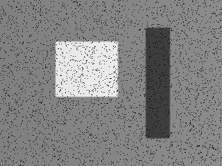
Therefore the final output takes the median + Gaussian cascade (Figure 38.3): the first median pass clears away the spikes and any impulse that may have slipped through, and the second Gaussian pass further soothes the residual random jitter. This combination preserves the edges of the boss and groove while pressing the flat-region RMS below 2 μm, laying a clean foundation for the measurement to come.
38.3 3D Morphology: Hole Filling
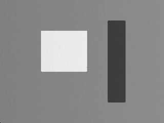
Filtering dealt with the “jitter” and the “spikes,” but did not touch the 3858 black holes — the invalid pixels are still holes. Hole filling is a job for morphology, and the idea is consistent with the 2D morphology of Chapter 8: use a closing operation (dilation followed by erosion) to fill in small-sized holes. On the height map, for each invalid pixel we inspect its 8-neighborhood, and if the number of valid neighbors reaches a threshold, we fill it with the median of those valid neighbors, iterating for several rounds — this is equivalent to letting the valid region “grow” inward a few rings, gradually closing up the isolated small holes while leaving the large continuous gaps untouched.
The experimental result is crisp and clean: the invalid pixels drop from 3858 to 1 — the closing operation filled 3857 small holes (Figure 38.4). Most of the 5% invalid pixels are scattered holes of 1 to 3 pixels, and a few rounds of closing can gather them all up.
Why “closing” and not “opening”? The closing operation fills the dark holes inside the foreground (the valid region), which is exactly the invalid pixels we want to fill; the opening operation, by contrast, erases small bright spots, a use of an entirely different kind. The choice of morphological operator always depends on which — the “hole” or the “spike” — is the object you want to eliminate.
But hole filling must be done with vigilance. Small holes can be filled, but what you fill a big hole with is fake data. Closing fills a hole by interpolating from the surrounding valid points, which carries the implicit assumption that “the surface beneath this hole is continuous with its surroundings.” For scattered holes of a few pixels, this assumption essentially holds, and the filled height is credible enough; but once you face a large continuous gap — say, a blind zone left where the laser was wholly occluded by a deep groove or steep wall — forcibly interpolating from the surrounding heights amounts to fabricating, out of thin air, a stretch of surface that was never measured at all. This is the same reasoning as the “better missing than fabricated” dilemma in Chapter 33: the missing data itself often carries information (there is a deep structure here, there is an abnormal reflection here), and mindlessly filling it flat instead erases the genuine signal. So the closing operation in this section deliberately sets the constraint that it “fills only when the number of valid neighbors reaches a threshold,” letting it fill only small holes and pass over large ones — and that 1 remaining invalid point is precisely the embodiment of this restraint.
38.4 3D Sampling
After denoising and hole filling, the surface is clean, but there are still too many points. This section addresses the “too dense” problem. Voxel grid downsampling is the most commonly used means of point cloud downsampling: cut 3D space into small cubes of fixed edge length (voxels), replace all points that fall into the same voxel with one representative point (usually the centroid), and the point density is thereby uniformly thinned out. Its benefit is “spatial uniformity” — no matter where the original point cloud is dense and where it is sparse, the output point spacing is uniformly constrained by the voxel edge length, with no local over-density.
Taking a voxel edge length of 0.4 mm, this chapter’s range image goes from 76799 valid points down to 4901, a 15.7× reduction (Figure 38.5). The key is that this reduction barely harms the structure: the densely packed points on the flat base already have similar heights and fall into the same batch of voxels, so collapsing them into representative points loses almost no information; while the edges of the boss and the groove, because their heights span different Z voxel layers, keep their points, and the edge density is relatively prominent by comparison. Figure 38.5 clearly shows this: the flat region is sparse in points, yet the contour lines of the groove and the boss remain dense — the structural information has been preserved intact.

Voxel sampling is not the only kind of downsampling. Uniform sampling takes every n-th point at a fixed stride, simple but liable to miss details; voxel sampling takes a representative point per spatial cell, with uniform density; curvature-adaptive sampling thins aggressively in flat regions and keeps more in high-curvature regions (edges, corners), saving the most points while best preserving structure, at the cost of having to first estimate normals and curvature. The three are chosen according to “whether you need to preserve detail” and “whether you can afford the precomputation.”
Why must 3D always be downsampled? Because downstream algorithms are extremely sensitive to point count. The ICP in registration (Chapter 39) must search for the nearest neighbor of every point in every round; running ICP or feature matching on a million-point cloud means a million kd-tree queries per single round, and after dozens of rounds the computation flat-out explodes; template matching and surface registration are the same. Cutting the point count by an order of magnitude or two first, before doing this heavy work, is often the key step that turns “won’t run” into “real-time.” Of course downsampling is also scene-dependent: for localization and registration, the downsampled result is both fast and stable; but for high-precision volume or dimensional measurement, you should use full resolution — a trade-off we will encounter again in the next section’s industry case.
38.5 3D Thresholding and Segmentation
The last step of preprocessing is often to separate the “region of interest” from the background and hand it off to subsequent measurement. The simplest and most direct 3D segmentation is height thresholding, an idea exactly like the 2D gray-value thresholding of Chapter 7: set a height threshold, classify everything above it as the target and everything below it as background. This chapter separates the boss from the base by “height > 1200 μm” — the base sits around 1000 μm, the boss rises 400 μm to about 1400 μm, and the 1200 μm line falls cleanly between the two.
The result is nearly perfect: the segmentation yields 7197 pixels, while the boss ground truth (GT) is 7200 pixels, with 0 false positives (FP) and 3 false negatives (FN), and an intersection-over-union of IoU = 0.9996 (Figure 38.6). All 3 false negatives are on the boss edge — where the height happens to sit right at the threshold and, after being slightly smoothed by filtering, dipped below the line, an acceptable boundary effect. Achieving this kind of precision owes much to the groundwork of the previous sections: filtering first removed the spikes that would have caused massive misclassification, and hole filling then filled the holes inside the boss that would otherwise have been judged as background, so that threshold segmentation could come out this clean.
Height thresholding is only the starting point of 3D segmentation. When the height difference between target and background is not obvious, or when the regions to be separated are coplanar, you need more advanced means: region growing clusters adjacent points into patches by the continuity of normals or curvature, and plane segmentation (RANSAC plane fitting) directly extracts plane primitives one by one from the point cloud (echoing the primitive fitting of Chapter 41). But for the most common industrial targets of the “boss that rises a notch / groove that drops a notch” kind, a single height threshold is often enough — simple and reliable.
38.6 SciVision Implementation
The usability of this chapter’s corresponding SciVision 3D module varies greatly in testing on this machine; it is recorded faithfully below for engineering trade-offs.
- SciSv3DFilter’s
Median/Gaussianare usable and NaN-aware (they correctly skip invalid pixels), consistent with the hand-written implementations; - SciSv3DMorphology’s
Close(closing for hole filling) is usable; - SciSv3DThreshold is inert on this machine —
ManualThresholdreturns rc = 0 but produces empty output, so segmentation has to be done yourself; - SciSv3DSampling’s
Samplingoverload on the range image fails (returns 123403001), and switching to the point cloud’sVoxelSamplingis non-deterministic across runs (the same input yields a drift of 4821/4821/0 over three runs), which is unreliable.
Therefore the main line of this chapter uses entirely hand-written, NaN-aware, deterministic implementations to produce the figures and numbers, while the various SDK 3D modules are placed in an isolated subprocess as probes, corroborating their return codes and usability (the 3D modules on this machine occasionally throw a 0xC0000005 access violation, so they are isolated to avoid dragging down the main flow). Below are the two most critical hand-written snippets. The NaN-aware median filter keeps the center invalid if it is invalid, otherwise takes the median of only the valid neighbors:
// 3x3 NaN-aware median: suppresses spikes, preserves edges; invalid points neither participate nor get contaminated
for (int dy = -r; dy <= r; ++dy)
  for (int dx = -r; dx <= r; ++dx) {
    double v = h[(yy)*W + xx];
    if (valid(v)) w.push_back(v);   // collect only valid neighbors
  }
std::sort(w.begin(), w.end());
out[y*W + x] = w[w.size() / 2];     // median
Voxel grid downsampling quantizes \((X,Y,Z)\) to a voxel key and keeps one representative point per voxel:
long long ix = floor(X / L), iy = floor(Y / L), iz = floor(Z / L);
long long key = (ix*100003LL + iy)*100003LL + iz;   // voxel key
Vox& g = grid[key];                                 // merge points falling into the same voxel
if (g.n == 0) { g.rx = x; g.ry = y; }               // first point as representative
g.sx += X; g.sy += Y; g.sz += Z; ++g.n;
The complete runnable project is located at code/point_cloud_preprocessing/; readers can change the noise level, voxel edge length, and segmentation threshold to reproduce all the figures and numbers themselves.
Industry Case: Holes and Downsampling in 3D Solder Paste Inspection
SPI (Solder Paste Inspection) uses a 3D camera to measure the volume of solder paste on each pad. The specular reflection of solder paste prevents the laser from being returned, leaving a large number of invalid pixels — and if you integrate the data with holes directly, the holes are treated as zero height, the volume is systematically underestimated, and a flood of “insufficient paste” false alarms results. The correct approach is to first fill the measurement holes with morphological closing, then integrate. But hole filling has an iron rule: you may only repair “measurement holes,” never fill in “process holes” — somewhere with no paste printed at all (a missed print) is a genuine process defect and must never be filled by the hole-filling algorithm; distinguishing the two kinds of holes relies on a joint judgment of size, position, and surrounding morphology. On downsampling: measuring volume requires full resolution to preserve precision, while locating pad positions on a large board is fast and accurate enough with a downsampled point cloud. The lesson is just one sentence: at every step of preprocessing, you must distinguish “repairing a measurement defect” from “erasing a genuine signal.”
38.7 Summary
The key points of this chapter can be distilled as follows.
- Preprocessing is the 3D counterpart of 2D enhancement. The four steps of denoising, hole filling, downsampling, and segmentation correspond respectively to spatial filtering, morphology, sampling, and thresholding — swap “gray value” for “height,” and most of the mature 2D algorithms can be directly transplanted to the range image for reuse.
- Invalid pixels must never enter the computation as 0. Every operator step in 3D must be NaN-aware, counting only valid neighbors; otherwise a single hole will drag the surrounding true heights down into a fake trough.
- The median removes spikes, the Gaussian smears them. The lesson of Chapter 6 replays in 3D: the median presses the spikes down to just 5 (RMS 32.09 → 2.28 μm), while the Gaussian paints the spikes into bumps (14 residual); the median + Gaussian cascade achieves 1.61 μm.
- Hole filling must distinguish measurement defects from genuine signals. Closing is very effective at filling small holes (3858 → 1), but what forced interpolation fills a large gap with is fake data — the same dilemma as “better missing than fabricated” at occlusions.
- Downsampling is the prerequisite for 3D to run. The voxel grid reduces 76799 points to 4901 (15.7×) while preserving the structural edges; ICP/matching on a million points will explode without downsampling first, but high-precision measurement still needs full resolution.
For a more systematic treatment of filtering, morphology, and segmentation of 3D data in industrial inspection, see further the book by Steger et al. (Steger, Ulrich, and Wiedemann 2018). This chapter’s statistical outlier removal (SOR) with its “neighborhood average distance \(\mu+t\sigma\)” criterion comes from the denoising pipeline Rusu et al. proposed while building point-cloud object maps for household scenes (Rusu et al. 2008); the open-source reference implementation of voxel-grid downsampling and the other operators above is surveyed in the Point Cloud Library (PCL) overview (Rusu and Cousins 2011).