11 Frequency Domain Processing and the FFT

In the previous chapters we have worked entirely in the spatial domain: an image is an array of pixels, filtering is a weighted operation over a neighborhood, and every question revolves around “what is the gray value where.” This chapter switches perspective — the frequency domain cares not about “where” but about “how fast”: how rapidly does the image’s gray value vary across space? A slowly undulating background is low frequency; sharp edges and fine, dense textures are high frequency. This perspective is no mathematical game — it solves practical problems that leave the spatial domain helpless. Imagine a production-line image contaminated by periodic electromagnetic interference: the entire image is overlaid with fine diagonal stripes. In the spatial domain this interference is everywhere, entangled with the image content; mean filtering cannot wipe it away, and median filtering is equally powerless. But in the frequency domain, this whole-image interference collapses into two isolated bright dots — carve them out with a small circle, and the interference vanishes almost losslessly. This chapter will demonstrate this “killer” application in full; but first, let us learn the language of the frequency domain.

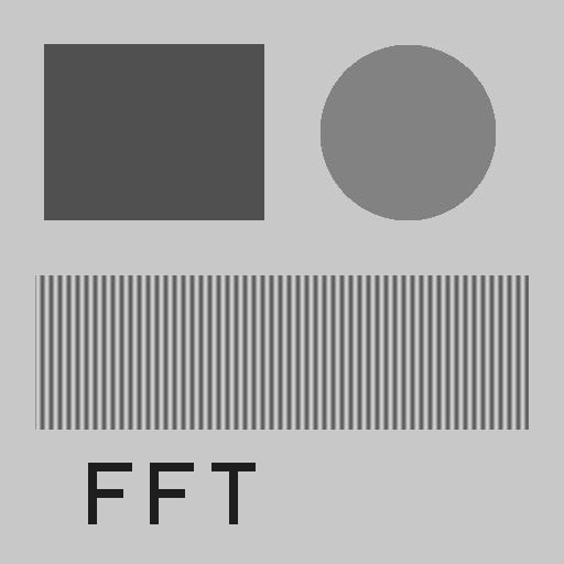
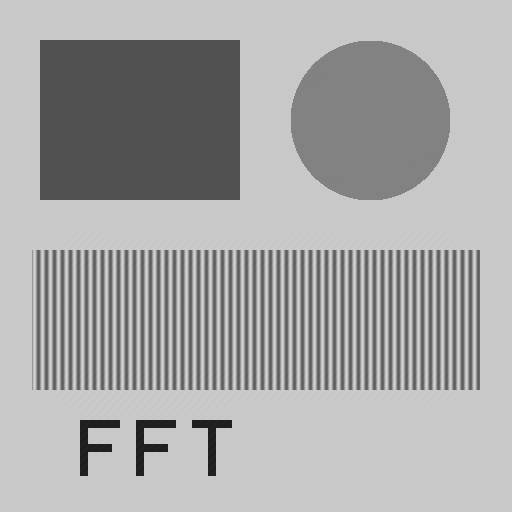
Our experimental scene (Figure 11.1) is a 512×512 synthetic image: a large dark rectangle and a large circle provide low-frequency blocky structure, the middle band is a vertical stripe pattern with a period of exactly 8 px (a high-frequency component of known frequency), and below it sit the dot-matrix letters “FFT” (text-like detail). Each component will leave a recognizable signature in the spectrum.

Figure 11.1: The 512×512 experimental scene: a large rectangle and a large circle (low-frequency blocky structure), a vertical stripe band with an 8 px period (known high frequency), and the dot-matrix text “FFT” (detail component).

11.1 The Two-Dimensional Fourier Transform

The core idea of the Fourier transform is that any signal can be decomposed into a superposition of sinusoids of different frequencies. For a \(W\times H\) discrete image \(f[n,m]\) (with \(n\) the row and \(m\) the column), the 2D Discrete Fourier Transform (DFT) is defined as

\[ F[u,v] = \sum_{n=0}^{H-1}\sum_{m=0}^{W-1} f[n,m]\, e^{-j 2\pi \left(\frac{um}{W} + \frac{vn}{H}\right)}, \]

where \(u,v\) are the frequency indices in the horizontal and vertical directions. The inverse DFT superposes the frequency components back into the image:

\[ f[n,m] = \frac{1}{WH}\sum_{u=0}^{W-1}\sum_{v=0}^{H-1} F[u,v]\, e^{+j 2\pi \left(\frac{um}{W} + \frac{vn}{H}\right)}. \]

Computing the DFT directly from the definition takes \(O(N^2)\) operations (\(N=WH\)) — about \(7\times 10^{10}\) for a 512×512 image, which is unacceptable. The Fast Fourier Transform (FFT) exploits the symmetry of the twiddle factors to bring the complexity down to \(O(N\log N)\). This is precisely what makes frequency-domain methods practical, and it is why this chapter’s experiments use image sizes that are integer powers of 2.

\(F[u,v]\) is a complex number, and in engineering practice it is almost always split into two more intuitive quantities. The magnitude spectrum \(|F[u,v]| = \sqrt{\mathrm{Re}^2 + \mathrm{Im}^2}\) answers “how much of the sinusoidal component at frequency \((u,v)\) is present”; the phase spectrum \(\arg F[u,v]\) answers “where that component sits” — the same set of sinusoids, given different phases, superposes into a completely different image. Filtering operations work mainly on the magnitude, but when reconstructing the image the phase must be preserved exactly as it is, or the image structure will become unrecognizable.

One frequency component deserves to be singled out: at \(u=v=0\) the exponential term is identically 1, so \(F[0,0] = \sum f[n,m]\) — exactly the sum of all gray values in the image, i.e. \(WH\) times the average gray level. This is the DC component — the statement in Chapter 6 that “the sum of the kernel weights equals the DC gain” originates exactly here: a filter with DC gain 1 leaves \(F[0,0]\) unchanged, and therefore leaves the image’s average brightness unchanged.

Plotting \(|F|\) directly as an image shows almost nothing: the energy of the DC component is orders of magnitude larger than that of nearly all high-frequency components, so under a linear gray mapping the entire spectrum is essentially black except for a single point at the center. The standard practice is to display the log spectrum \(\log(1+|F|)\), which compresses the enormous dynamic range into an interval the eye can resolve — every spectrum in this chapter is plotted this way.

11.2 Reading the Spectrum

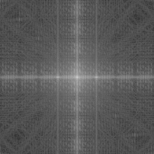
Figure 11.2 is the log magnitude spectrum of the experimental scene (with the DC component shifted to the image center). Reading a spectrum is a skill you can pick up quickly — let us identify each feature against the scene.

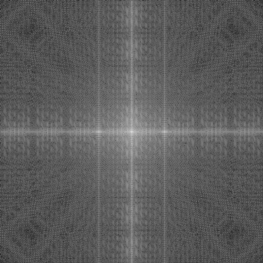
Figure 11.2: Log magnitude spectrum of the experimental scene (DC centered). The bright central blob is low-frequency energy, the bright horizontal/vertical cross comes from the axis-aligned edges of the rectangle and the stripe band, and the symmetric pair of dots at ±64 on the horizontal axis is the signature of the 8 px vertical stripes.

The bright central blob: low-frequency energy. Slowly varying blocky structures like the large rectangle and the large circle concentrate nearly all of their energy near the center.
The bright horizontal and vertical cross: the rectangle’s horizontal/vertical edges and the stripe band’s horizontal boundaries are all “abrupt transitions along one direction,” and in the frequency domain an abrupt transition spreads out into a line perpendicular to the edge.
A symmetric pair of bright dots on the horizontal axis: a pure periodic stripe pattern is, in the frequency domain, just a pair of impulses — this is the most important correspondence in this chapter.

The position of this pair of dots can be predicted first, then verified. A stripe pattern with period \(T\) pixels repeats exactly \(W/T\) times across an image of width \(W\), so its spectral peak appears at horizontal frequency index

\[ u = \frac{W}{T} = \frac{512}{8} = 64 \]

— that is, at \(\pm 64\) on either side of the center. In the experiment we exclude the central low-frequency region and search the whole spectrum for the maximum magnitude; the measured peak position is \((\Delta u, \Delta v) = (-64, 0)\) — an exact hit on the prediction. This “known period → spectral peak position” conversion is a directly usable weapon when troubleshooting periodic interference on a production line: measure the pixel period of the interference stripes, and you know exactly where in the spectrum to look for them.

Conjugate symmetry: the spectrum of a real-valued image satisfies \(F[-u,-v] = F^*[u,v]\), so the magnitude spectrum is symmetric about the center — this is why spectral peaks always appear in pairs. When we do notch filtering later, the conjugate peak of every interference peak must be handled along with it, or the result of the inverse transform will no longer be a real image.

11.3 Frequency-Domain Filtering

The theoretical cornerstone of frequency-domain filtering is the convolution theorem: convolution in the spatial domain is equivalent to pointwise multiplication in the frequency domain,

\[ f * h \;\longleftrightarrow\; F \cdot H. \]

This means that all of the linear filtering of Chapter 6 can be carried out in the frequency domain: take the FFT of the image, multiply the spectrum pointwise by the filter’s frequency response \(H\), then apply the inverse transform. The two routes are mathematically identical; the engineering trade-off is computational cost. Spatial convolution with a \(K\times K\) kernel costs \(O(K^2)\) multiply-adds per pixel, while the frequency-domain route’s cost is independent of kernel size — use the spatial domain for small kernels, and the frequency domain for large ones (tens of pixels and up).

The simplest frequency-domain filter is the ideal lowpass filter: \(H=1\) within radius \(D_0\) of the DC center, \(H=0\) outside, zeroing out the high frequencies in one clean cut; the ideal highpass is exactly the opposite. We run the experiment with a cutoff radius of 30 px (normalized frequency \(30/256 \approx 0.1172\)); the results are shown in Figure 11.3.

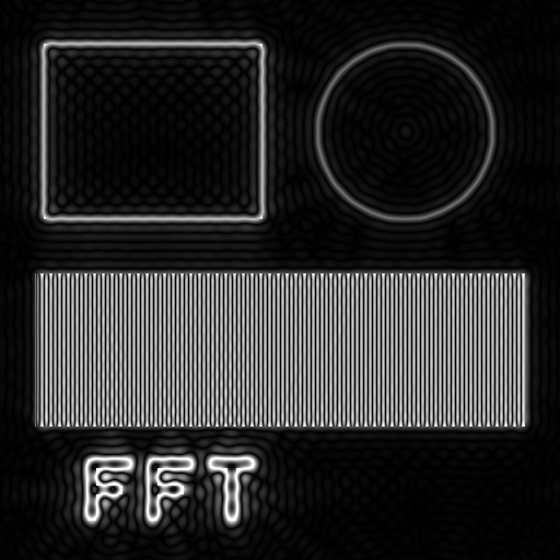
The lowpass result confirms the prediction: the stripe frequency of 64 lies far outside the cutoff radius of 30, and the entire stripe band is flattened into uniform gray. But notice the concentric ripples around the rectangle, the circle, and the text — this is Gibbs ringing, the price the ideal filter must pay. The cause is clear-cut: a hard rectangular truncation in the frequency domain has the sinc function as its spatial-domain counterpart, and the sinc has oscillating sidelobes that trail on endlessly; by the convolution theorem, multiplying in the frequency domain equals convolving in the spatial domain with this long-tailed kernel, so every edge gets dragged out into a train of ripples. For this reason the ideal filter is rarely used in engineering practice; one uses Gaussian or Butterworth filters instead — their frequency responses transition smoothly, their spatial-domain kernels no longer oscillate, and the only cost is a cutoff edge that is not quite as “sharp.”

The lesson of ringing fits in one sentence: the harder you cut in the frequency domain, the longer the smear in the spatial domain. This is the flip side of the same coin as Chapter 6’s observation that “the Gaussian kernel’s frequency response has no sidelobes, so its smoothing is clean.”

The highpass result likewise speaks the language of the spectrum: once the low frequencies within radius 30 are zeroed, the blocky structures are reduced to their edge outlines (edges are high frequency), while the stripe band survives almost untouched — its frequency of 64 is above the cutoff of 30, inside the highpass passband. Highpass filtering is therefore often used as a means of edge enhancement and background suppression.

11.4 Notch Filtering of Periodic Noise

Now for this chapter’s central demonstration. We superimpose a diagonal sinusoidal interference \(40\sin\!\big(2\pi(r+c)/8\big)\) onto the scene (period about 5.7 px along the diagonal), simulating periodic stripe contamination from electromagnetic interference or mechanical vibration. The RMSE between the noisy and clean images is 28.13 — consistent with the theoretical value \(40/\sqrt{2} \approx 28.3\) (the RMS amplitude of a sinusoid). Spatial-domain filtering is powerless against it: the interference’s spatial frequency is quite close to that of the useful 8 px stripes in the scene, and any smoothing strong enough to suppress the interference would wipe out the useful stripes along with it.

But in the frequency domain, this interference is just two dots. Figure 11.4 shows the complete pipeline.

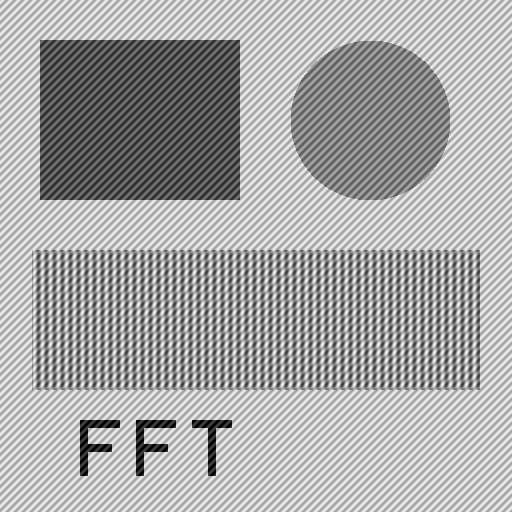
Predict first: the interference has a period of 8 px along both the row and column directions, so the spectral peaks should appear at \((\pm 512/8, \pm 512/8) = (\pm 64, \pm 64)\). Searching the spectrum yields \((-64, -64)\) and its conjugate peak \((+64, +64)\) — another exact hit. Next comes the four-step notch filtering procedure:

Take the FFT of the noisy image (DC centered);
Exclude the central low-frequency region and search for the interference peak of maximum magnitude;
Zero out the complex spectrum inside a small circle of radius 5 px centered on the peak, and treat the conjugate peak the same way;
Inverse-transform back to the spatial domain and clamp to [0, 255].

The result (Figure 11.4 (c)) is nearly indistinguishable from the original: the RMSE drops from 28.13 to 0.61, more than 98% of the interference energy is eliminated, and the useful vertical stripes (peaks at \(\pm 64\) on the horizontal axis, far away from the interference peaks) are left without a scratch. This is exactly what makes frequency-domain methods irreplaceable: two components can be very close in spatial-domain “speed,” yet as long as their direction or period differs slightly, they are separate points in the spectrum — spatial filtering cuts by “speed” alone, while a frequency-domain notch strikes precisely where you aim. The residual 0.61 comes from the small amount of the image’s own energy lost inside the carved-out circles — a reminder that for the notch radius, smaller is safer.

11.5 The Sampling Theorem Revisited

Armed with the language of the frequency domain, the aliasing intuition from Chapter 1 — “sample each period at least twice” — can finally be upgraded to a formal statement. The Nyquist sampling theorem: as long as the signal’s highest frequency component is below half the sampling frequency, the original signal can be perfectly reconstructed from its samples. The frequency domain makes it clearest — sampling replicates the original signal’s spectrum periodically at intervals of the sampling frequency, and once the signal’s bandwidth exceeds half the sampling frequency, adjacent spectral replicas shift into overlap: high-frequency components masquerade as low frequencies and mix into the signal, with no way to separate them after the fact. This also explains the rule from Chapter 10 that an image must be smoothed before shrinking: downsampling amounts to lowering the sampling frequency, and pre-filtering means trimming the spectrum down to within the new Nyquist limit first — better to lose detail than to let detail turn into spurious low-frequency artifacts.

11.6 SciVision Implementation

All of this chapter’s experiments are carried out by the SCIMV::SciSvFFT class; the core calls are as follows:

SCIMV::SciSvFFT fft;
SciImage fftImg;
// mode=0: shift the DC component to the spectrum center; fftImg is a 2-channel 32F image with interleaved real/imaginary parts
fft.ApplyFFTGeneric(src, 0, &fftImg, NULL);

// Ideal lowpass/highpass: frequency is the normalized cutoff (relative to the half-width W/2), 0.1172 → measured radius 30.0 px
float cutoff = 30.0f / (512 / 2);
SciImage lp;
fft.GenerateLowpass(cutoff, 0, 512, 512, &lp);

// The convolution theorem in action: multiply the spectrum pointwise by the filter
SciImage fftLP, out32;
fft.ApplyFFTConvolution(fftImg, lp, &fftLP);
// Inverse transform: always request SCI_IMAGE_32F, then clamp to [0,255] yourself
fft.ApplyIFFTGeneric(fftLP, 0, &out32, true, SCI_IMAGE_32F);

The complex spectrum output by ApplyFFTGeneric can be read and written directly through ImageData() and Step() — the real and imaginary parts at row \(r\), column \(c\) sit at float offsets r*stride + 2*c and r*stride + 2*c + 1. The notch filtering of Section 11.4 is implemented exactly this way, manually zeroing the complex values inside the two small circles — the SDK provides no ready-made notch interface, and none is needed.

There are three experimentally confirmed pitfalls in using this API, recorded as found:

IFFT output as 8U is min-max normalized: requesting 8-bit output directly stretches the gray values wholesale, and the roundtrip (FFT→IFFT) RMSE comes out at a staggering 33.62 — it looks like the algorithm is broken, but it is the normalization. Request SCI_IMAGE_32F to get the raw floating-point result and clamp it yourself, and the roundtrip RMSE is 0.0000 — the transform itself is lossless.
The magnitude image built into ApplyFFTGeneric is nearly all black: its imageMagnitude output uses linear normalization, the DC component dominates, and all other frequencies are invisible. The log spectrum \(\log(1+|F|)\) must be computed yourself from the complex data.
RemovePeriodicPatternsByFFT is unusable: this interface is explicitly marked “not implemented” in the header file; for periodic noise removal, do the notch filtering manually following this chapter’s procedure.

The complete project that generates all of this chapter’s images is located at code/fourier/; the predicted versus measured spectral peak positions are printed directly to the console.

Industry Case: Weave Patterns on Textile Surfaces

In a textile surface-defect inspection project, the fabric’s own warp-and-weft weave pattern was a strong periodic structure whose gray-level fluctuation far exceeded the defect signals — broken yarns, oil stains — leaving the defects nearly invisible in the raw image. Spatial filtering was caught in a dilemma: a small kernel could not filter the weave out cleanly, while a large kernel blurred the defects away together with the weave. Switching to a frequency-domain approach dissolved the problem — the weave’s fundamental frequency and its harmonics form a set of bright dot pairs at stable positions in the spectrum; applying a small-radius notch to each pair and inverse-transforming back to the spatial domain removed the weave wholesale, leaving the defects plainly visible in the residual image. The key lesson from on-site tuning was that for the notch radius, smaller is safer: defect energy is also distributed near the weave peaks, and while a larger radius filters the weave more thoroughly, it swallows defect energy and lowers detection contrast — size the notch to just cover the spectral peak.

11.7 Summary

The frequency domain answers “how fast”; the spatial domain answers “where”: the magnitude spectrum gives how much of each frequency component is present, the phase spectrum gives where they sit; the DC component \(F[0,0]\) is the sum of all gray values, and the log display \(\log(1+|F|)\) is the standard way to look at a spectrum.
Spectra can be read — and, better still, predicted: stripes with period \(T\) in an image of width \(W\) produce a conjugate peak pair at \(u=W/T\) — the 8 px stripes predicted ±64, and the measurement hit it exactly.
The convolution theorem \(f*h \leftrightarrow F\cdot H\) connects the two domains: use spatial convolution for small kernels, the frequency-domain route for large ones; a hard cut in the frequency domain invites Gibbs ringing (the sinc’s trailing tail), so engineering practice replaces ideal filters with smoothly transitioning Gaussian/Butterworth ones.
Notch filtering is the specific cure for periodic interference: whole-image periodic contamination is just a few points in the spectrum; zero out small circles and inverse-transform — in the experiment the RMSE dropped from 28.13 to 0.61, something no spatial filter can achieve.
The Nyquist theorem, stated in frequency-domain terms: the signal’s highest frequency must be below half the sampling frequency, or shifted spectral replicas overlap and produce aliasing — this is the root reason pre-filtering is mandatory before downsampling.

The fast algorithm that made the FFT practical originates in the classic 1965 paper by Cooley and Tukey (Cooley and Tukey 1965), which cut the complexity of the DFT from \(O(N^2)\) to \(O(N\log N)\); the systematic treatment of the Fourier transform in digital image processing (including frequency-domain filtering and notch filters) is the textbook by Gonzalez and Woods (Gonzalez and Woods 2018). For a systematic treatment of frequency-domain methods in industrial image processing (including optimal filtering and frequency-domain features), see the book by Steger et al. (Steger, Ulrich, and Wiedemann 2018).