12 Advanced Enhancement

Up to this point, most of what we have done to images is “repair”: removing noise (Chapter 6), flattening illumination (Chapter 4), stretching gray values into a suitable range. What these operations share is restoration — whatever the image was supposed to look like, we patch it back to that state. This chapter turns in a different direction: reinforcement. Some information truly is in the image, yet too weak for downstream algorithms to use directly — edges flattened by the softening of the lens and defocus, dark-region detail drowned in readout noise, bright-region detail crushed into a sheet of white by the sensor’s full-well and quantization ceiling. The two tools of this chapter exist precisely for this: sharpening stands the flattened edges back up, compensating for the MTF losses of the imaging chain; high dynamic range (HDR) imaging uses multiple exposures to recover both the bright and dark ends of information that exceed the dynamic range of a single frame. Figure 12.1 gives a first look at the intuitive effect of the first tool: an edge softened by defocus is stood back up by unsharp-mask enhancement. As for shadows caused by uneven illumination, Chapter 4 has already discussed shading correction in detail, and we will not repeat it here.

(a) Softened scene (defocus simulated by a \(\sigma=1.5\) Gaussian)

12.1 Sharpening and the Unsharp Mask

The most classic — and most widely used — form of sharpening is unsharp masking. The seemingly self-contradictory name comes from the darkroom era: photographers deliberately printed a blurred (“unsharp”) copy of the negative as a mask and exposed it together with the original, and the result was, counterintuitively, a sharper photograph. The digital version takes only three steps: blur the image once with a low-pass filter, subtract the blurred version from the original to obtain a detail layer, then add the detail layer back in proportion:

\[ g = f + \lambda\,\big(f - G_{\sigma} * f\big), \]

where \(G_{\sigma} * f\) is the Gaussian blur of \(f\) (in Chapter 6 we used it to suppress noise; here we use it to separate frequency components) and \(\lambda\) is the enhancement strength. The logic of the operation is perfectly direct: the Gaussian blur keeps the low frequencies and filters out the high ones, so \(f - G_{\sigma}*f\) is exactly the high-frequency part that was filtered away — edges, thin lines, texture; multiplying it by \(\lambda\) and adding it back to the original is equivalent to amplifying the image’s high-frequency content by a factor of \(1+\lambda\). \(\lambda\) is the “high-frequency gain knob”: \(\lambda=0\) passes the image through unchanged, and the larger \(\lambda\), the stronger the edge contrast. The \(\sigma\) of the blur kernel decides “how fine counts as detail” — it should be comparable to the blur scale being compensated.

Sharpening compensates for the MTF attenuation caused by lens aberrations, slight defocus, and the like (Chapter 3), but it cannot create information: it can only amplify whatever high-frequency residue still survives, together with the noise inside it. If the MTF at some spatial frequency has already decayed to zero, the detail layer contains no trace of it whatsoever, and no value of \(\lambda\) will conjure it back. Sharpening is an “amplifier”, not a “restorer”.

We demonstrate with a controlled experiment. Take the same synthetic scene as in Chapter 6 (bright background 180, dark rectangle 60, one thin bright line 2 px wide at 250), and first soften it with SciVision’s Gaussian filter (\(9\times 9\), \(\sigma=1.5\)) to simulate a slightly defocused lens: this yields Figure 12.1 (a), where the edges are already visibly fuzzy. Then, using the same Gaussian (\(9\times 9\), \(\sigma=1.5\)) as the blur term of the unsharp mask, we enhance with \(\lambda=1.0\) and obtain Figure 12.1 (b): the step edges become crisp again, and the contrast of the thin bright line recovers substantially.

12.2 Overshoot and Ringing

Since \(\lambda\) is a gain knob, would turning it up make things even sharper? Figure 12.2 (a) shows the result at \(\lambda=4.0\): the edges are indeed “sharper”, but a glaring bright halo floats around the dark rectangle, and the inside of the rectangle is rimmed with a band that is too dark. These are overshoot and undershoot — the sharpening “pushes too hard” upward and downward on the two sides of the step, driving the gray values past their original plateau levels. When the enhancement kernel has a steep frequency cutoff, the overshoot can also repeat as a decaying oscillation, called ringing.

Numbers are the most persuasive. We extract the gray-level profile along row 180, columns 90–150 (cutting straight across the left edge of the dark rectangle, with nominal gray values of 180 on the bright side and 60 on the dark side); the three curves are plotted in Figure 12.2 (b), with statistics as follows:

Table 12.1: Overshoot statistics of the row-180 profile (columns 90–150); nominal gray values 180/60

Profile	min	max	Overshoot / undershoot
Softened original	58	178	+0 / −2
\(\lambda=1.0\)	56	185	+5 / −4
\(\lambda=4.0\)	36	213	+33 / −24

At \(\lambda=1.0\) the overshoot is only +5/−4 gray levels — the same order as the image noise and invisible to the eye; at \(\lambda=4.0\) it surges to +33/−24, pushing out “false plateaus” of roughly 30 gray levels on each side of the edge.

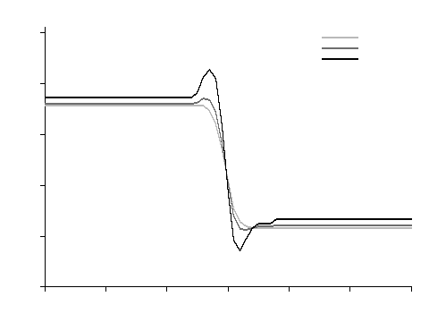
Overshoot is by no means merely an aesthetic issue; it does real damage to both measurement and inspection. For measurement: the caliper tools of Chapter 20 locate edges at the derivative extrema of the gray-level profile; overshoot changes the shape of the profile on both sides of the edge, the derivative curve is distorted accordingly, and the edge positions found shift systematically — you thought sharpening made the edge “easier to find”, when in fact it “moved the edge”. For inspection: to blob analysis or threshold segmentation, the bright halo around a dark workpiece is a ring of genuinely existing high-brightness area, enough to trigger a false defect alarm; conversely, the dark rim inside a bright region may be misjudged as a crack. Hence the rule for choosing \(\lambda\): extract edge profiles on representative samples, increase \(\lambda\) until the overshoot amplitude approaches the image noise amplitude, and give it no more. Once the overshoot is buried in the noise, it has no systematic effect on downstream algorithms; in this example \(\lambda=1.0\) (overshoot +5, the same level as the noise) passes, while \(\lambda=4.0\) is far over the line. Also watch out for saturation: once overshoot is clipped at 0 or 255, the original gray-level information is lost for good.

12.3 High Dynamic Range and Exposure Fusion

The second kind of “weak information” problem lies in dynamic range: the ratio of irradiance between the brightest and darkest parts of the scene exceeds what a single frame can record. The ceiling comes from the sensor’s full-well capacity and 8-bit quantization (Chapter 3, Chapter 1); the floor comes from readout noise. The result is a dilemma: expose for the highlights and the shadow detail sinks into noise; expose for the shadows and the highlights wash out to solid white. The workpiece contour next to a welding pool, or characters etched on polished metal, are typical victims.

The idea of multi-exposure fusion (exposure fusion) is: if the dynamic range is not enough, shoot several frames and combine them. Capture the same static scene at multiple exposure levels — short exposures keep the highlights, long exposures scoop up the shadows — then merge the information pixel by pixel into a single estimated irradiance map. Under the linear-response assumption (pixel value \(v_i \approx E \cdot t_i\), where \(t_i\) is the relative exposure), every frame gives one observation \(v_i/t_i\) of the irradiance, and a weighted average yields the estimate:

\[ \hat E(p) = \frac{\sum_i w(v_i)\, v_i / t_i}{\sum_i w(v_i)}, \qquad w(v) = \min(v,\, 255-v) + \varepsilon . \]

This is a simplified form of Debevec-style irradiance recovery, and \(w\) is the triangle weight: the weight is largest when the pixel value sits in the middle and falls toward zero as the value approaches 0 or 255.

The intuition behind the triangle weight is an election with vote screening: each exposure frame casts one vote on the pixel’s irradiance, but votes from too-dark pixels don’t count (the signal is drowned in noise, so \(v_i/t_i\) is wildly unreliable), and votes from too-bright pixels don’t count either (already clipped to saturation, so \(v_i\) simply does not equal \(E\cdot t_i\)). Only frames with a moderate exposure get a say — and for any point in the scene, some exposure level is bound to be just right, which is the entire point of taking multiple exposures.

The recovered \(\hat E\) exceeds the 8-bit range, so a final tone mapping step compresses it back into the displayable interval. This chapter uses the simplest global \(\gamma\) mapping: \(\text{out} = 255\,(\hat E/\hat E_{\max})^{1/2.2}\), where \(\gamma=1/2.2\) lifts the shadows and compresses the highlights, roughly matching human visual perception.

The irradiance field of the experimental scene is constructed as follows: a mid-gray background of 110; in the upper-left bright region, hidden vertical stripes of 252/272 (contrast 20, but with the peak above the 8-bit ceiling of 255); in the lower-right dark region, hidden vertical stripes of 14/24 (contrast 10, hugging the noise floor). We expose at three gain levels, ×0.25 / ×1.0 / ×4.0, each clipped to [0,255] with \(\sigma=2\) readout noise added (fixed seeds 11/22/33 for reproducibility), giving the three frames of Figure 12.3; fusing and tone-mapping yields Figure 12.4.

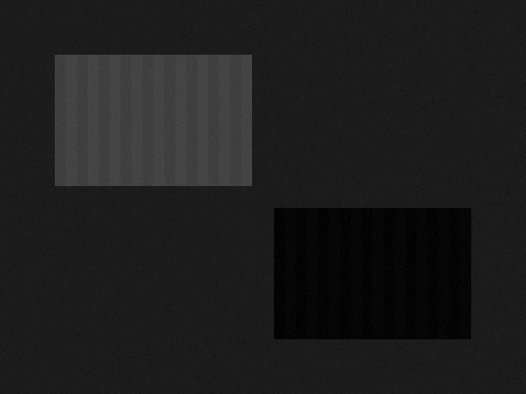
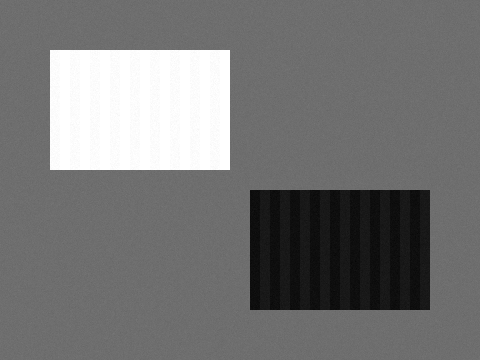
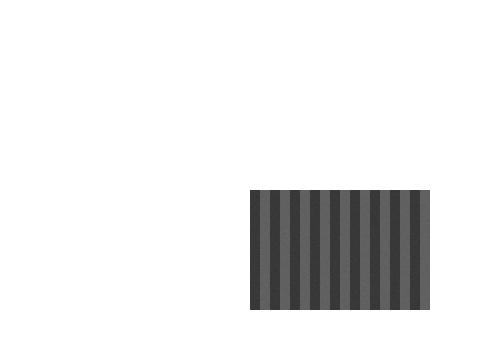
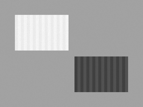
Figure 12.4: The HDR result after fusing the three frames and tone-mapping with \(\gamma=1/2.2\): the bright-region stripes and the dark-region stripes are clearly visible at the same time.

Beyond eyeballing, we compute the mean and standard deviation over the two stripe-detail patches (the standard deviation measures the visibility of the stripe contrast):

Table 12.2: Mean and standard deviation of the detail patches compared

Image	Dark patch mean / std	Bright patch mean / std
Short exposure (×0.25)	4.8 / 2.35	65.5 / 3.22
Mid exposure (×1.0)	19.0 / 5.40	253.5 / 2.03
Long exposure (×4.0)	76.0 / 20.13	255.0 / 0.00
HDR fusion	72.5 / 8.76	239.8 / 5.35

Read the table row by row: the short exposure’s dark-patch std of 2.35 is almost equal to the readout noise \(\sigma=2\) — the stripes are completely drowned; the mid exposure’s bright patch has mean 253.5 and std 2.03, the residue left after clipping; the long exposure’s bright-patch std is exactly 0.00 — total saturation, information reduced to zero. Of the four images, only the fused one retains clear stripe contrast in both detail patches at once (std 8.76 and 5.35, both several times the noise) — and that is precisely the value of HDR.

The experiment also throws in a bonus teaching point: the program prints a recovered irradiance peak of \(\hat E_{\max}=300.0\), while the scene’s ground truth is 272. The error comes from the short-exposure frame — its \(\sigma=2\) readout noise is amplified by a factor of \(1/0.25=4\) when converted back via \(v/t\); at the brightest pixels, where the mid and long exposures are both saturated, the short exposure is the only “valid vote” left, and its 4×-amplified noise is pushed straight onto the estimate. The reminder: what a short-exposure frame contributes to the irradiance estimate is amplified noise, and a more refined implementation would multiply the triangle weight by an additional exposure-time-dependent SNR weight.

12.4 SciVision Implementation

This chapter’s SDK usage needs to be disclosed honestly, because it is itself a lesson in engineering. We had originally planned to use SciSvEdgeEnhance::EnhanceEdges for sharpening and the SciSvHDR family for exposure fusion, but systematic testing while developing this chapter’s examples (v3.1) reached the following conclusions:

A full parameter sweep of SciSvEdgeEnhance::EnhanceEdges over type/offset/factor/brightness shows that every combination outputs a binary edge map of 0/255, not a sharpened “original + enhanced edges” image — it is actually an edge-map generator, and the name is misleading;
SciSvHDR::FusedPicture returns code 0 for grayscale input but crushes the entire dark region into dead black with a mean of about 0.1 (all detail lost); 3-channel input directly triggers an OpenCV cv::Mat assertion crash;
SciSvHDR::Compose, given 480×360 single-channel input, returns a 3-channel image cropped to 449×340;
SciSvHDR::ToneMapping(method=1) triggers an OpenCV cv::scaleAdd assertion and terminates the process outright (exit code 0xC0000409).

Therefore both the sharpening and the HDR fusion in this chapter are hand-written, and the SDK handles only the two things it does reliably: Gaussian filtering and image I/O. The Gaussian part is identical to Chapter 6:

SCIMV::SciSvFilter flt;
SciImage soft, blur;
flt.Gaussian(imgSharp, roi, &soft, 9, 9, 1.5, 1.5);  // simulate slight defocus
flt.Gaussian(soft, roi, &blur, 9, 9, 1.5, 1.5);      // blur term of the unsharp mask

The unsharp-mask core is a single line of arithmetic, executing \(\text{out} = \text{in} + \lambda(\text{in} - \text{blur})\) per pixel and clamping to [0,255]:

double v = in[i] + lambda * (in[i] - blur[i]);
out[i] = (unsigned char)(v < 0 ? 0 : (v > 255 ? 255 : (int)(v + 0.5)));

The implementation leaves pixels within 5 px of the image border untouched: subtracting the SDK Gaussian’s extrapolated border values from the original produces spurious differences, and enhancing them directly would frame the image with black-and-white border artifacts. The core of exposure fusion is equally compact — per pixel, accumulate the triangle-weighted votes over the three frames:

for (int k = 0; k < 3; ++k) {
    double v = (double)exps[k][i];
    double w = (v < 255.0 - v ? v : 255.0 - v) + 1e-3;  // triangle weight
    sw += w;
    se += w * v / t[k];     // t[] = {0.25, 1.0, 4.0}
}
E[i] = se / sw;             // then tone-map with gamma=1/2.2

The complete project is in code/advanced_enhancement/, and the file header preserves the full test record of the SDK defects above. The engineering lesson of this episode deserves bold type: every API of a commercial vision library must have its actual behavior verified with a golden experiment of known ground truth before it goes onto the line — construct a synthetic input whose result you can compute by hand, feed it to the API, and check the output. This is of one lineage with the methodology of Chapter 5, where calibration results are checked against a known target: the documentation is a promise; the experiment is the behavior.

Industry Case: HDR Code Reading on Laser-Etched Battery Shells

A battery-shell production line laser-etches batch codes onto polished aluminum shells, with the code-reading camera facing the highly reflective metal surface head-on: in a single exposure, either the character strokes saturate into solid white or the background is crushed into dead black — the contrast between characters and background never lines up, and the read rate hovered around 70%. The retrofit was to capture two exposure levels back-to-back at the same station (short exposure to keep the characters, long exposure to keep the background), fuse them into one frame by this chapter’s weighted scheme, and feed that to the code reader; the read rate rose above 99%. The cost was equally clear: one extra frame per product doubled the acquisition cycle time, and the line was forced to slow down. The alternative route evaluated later was to switch to a 12-bit high-dynamic-range camera, covering the full gray-level span in one frame — more expensive hardware, but no cycle-time penalty. The general conclusion of this case: for dynamic-range problems, think hardware first (deeper bit depth, larger full well), then algorithms (multi-exposure fusion) — the algorithmic route saves money but pays in time.

12.5 Summary

Enhancement is amplification, not restoration. The unsharp mask \(g = f + \lambda(f - G_\sigma * f)\) amplifies the high-frequency content by \(1+\lambda\), compensating the MTF attenuation caused by the lens and defocus, but detail whose MTF has already reached zero is beyond anyone’s saving, and the noise gets amplified along the way.
Bound \(\lambda\) by the overshoot. Extract profiles on representative edges and stop once the overshoot amplitude reaches the noise amplitude (in this chapter \(\lambda=1.0\) with overshoot +5 passes; \(\lambda=4.0\) with overshoot +33 is over the line); overshoot shifts caliper edge-finding systematically, and halos manufacture false defects.
When dynamic range falls short, make it up with multiple exposures. Irradiance recovery \(\hat E = \sum w(v_i)v_i/t_i \,/\, \sum w(v_i)\) with triangle weights — votes from too-dark and too-bright pixels don’t count; in the experiment only the fused image made the bright and dark details visible at the same time.
The noise of short-exposure frames is amplified by \(1/t\) (in this chapter \(\hat E_{\max}=300\) against a ground truth of 272); a refined implementation should add an SNR weight, and the engineering cost of fusion is a doubled cycle time — dynamic-range problems should first be weighed against the hardware route of a higher-bit-depth camera.
The behavior of commercial-library APIs must be verified with golden experiments. This chapter’s SDK sharpening and HDR interfaces were all either mislabeled or outright crashed; the final solution let the SDK do only Gaussian filtering and I/O, with the core algorithms hand-written — the documentation is a promise; the experiment is the behavior.

The standard treatment of sharpening methods such as the unsharp mask is the textbook by Gonzalez and Woods (Gonzalez and Woods 2018); the methodological origin of this chapter’s multi-exposure fusion is the work of Debevec and Malik at SIGGRAPH 1997, which recovers the camera response function and fuses a high-dynamic-range radiance map (Debevec and Malik 1997), while the complete framework of high-dynamic-range imaging — from acquisition through display to tone mapping — is the monograph by Reinhard et al. (Reinhard et al. 2010). For frequency-domain analysis of sharpening filters and more systematic gray-level transformation methods, see the book by Steger et al. (Steger, Ulrich, and Wiedemann 2018).