24 Contour Analysis

Blob analysis in Chapter 23 treats a target as a clump of pixels to be tallied — area, centroid, inertia axes — answering questions about “this lump of stuff”. But many industrial problems do not ask about the lump; they ask about the boundary: how far does this stamped part’s outline deviate from the drawing? Are there burrs, bumps, or missing material along the edge? The representation needed here is the contour — an ordered string of subpixel points laid out one after another along the target’s boundary. Ordered means you can walk the boundary point by point, segment it, and localize defect positions; subpixel means accuracy is not nailed down by the pixel grid. The contour is the high-resolution language of defect detection and shape measurement: the region tells you “how much” of a target there is, the contour tells you “what it looks like”.

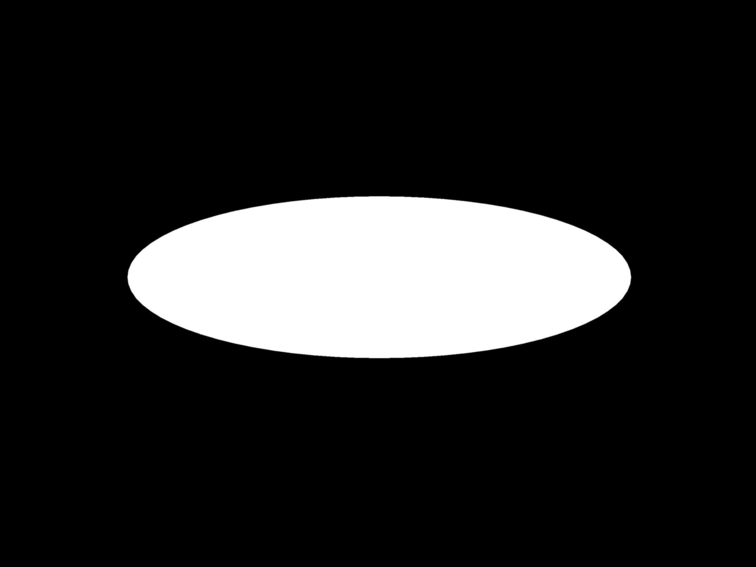
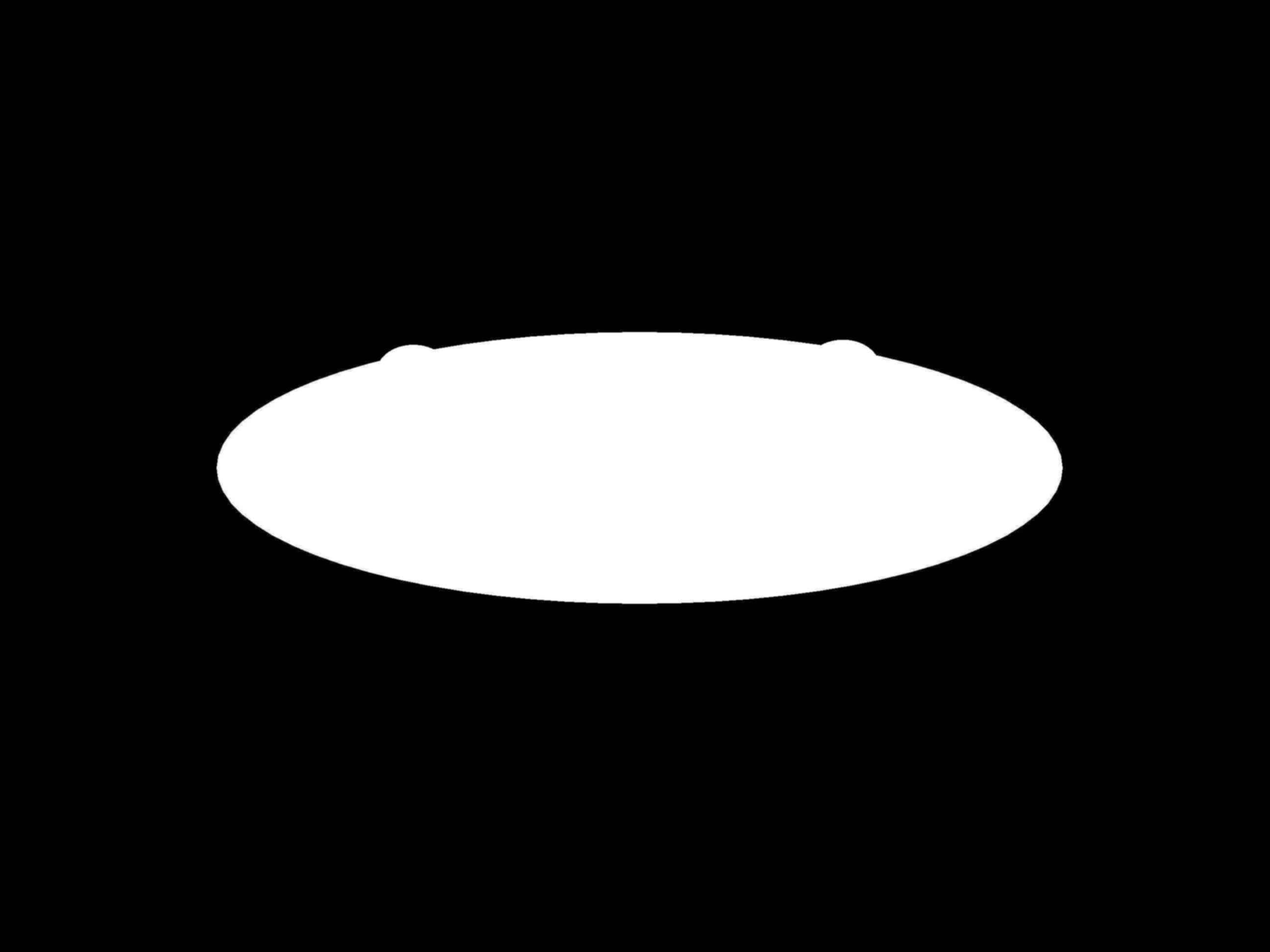
This chapter runs all of its experiments on a set of real industrial sample images (Figure 24.1): an ellipse-shaped workpiece imaged under backlight, yielding a 2592×1944 high-contrast silhouette — a bright white part against a pure-black background, with a narrow, steep gray transition band at the boundary, exactly the ideal input for subpixel contour extraction. There are three images: 001 is the standard part (the master), whose outline is a clean ellipse; 003 and 002 are two test parts, each carrying an edge defect — the top edge of 003 has two outward protrusions (excess-material defects), and the bottom edge of 002 has a single larger bump. We will extract all three parts’ contours, measure the master’s features, perform smoothing/resampling/segmentation operations on the master, and finally compare the test parts against the master point by point — letting the edge defects surface on their own.

24.1 Contour Extraction

Contour extraction stands on the shoulders of edge detection (Chapter 13): edge detection outputs an image of “which pixels are edges”, with no order among the pixels; contour extraction then does two more things — linking, stringing adjacent edge pixels into chains, and subpixel refinement, refining each point’s position along the chain from integer to subpixel (the same idea as the subpixel section of Chapter 13: parabolic interpolation over three magnitude samples along the gradient direction; the Steger-style curve extractor introduced there outputs subpixel line contours directly). The product of linking is an ordered point list, and the contour of a closed target joins head to tail into a loop.

The experiment extracts on the full-image ROI with subpixel Canny (hysteresis thresholds 20/40, smoothing coefficient 2.0). The key parameter is the minimum contour length minLen=600: the black background outside the silhouette has almost no gradient and produces virtually no stray contours, so the length filter is a safeguard — in the end each of the three parts retains just 1 closed contour, all with 3627 points: under the high-contrast silhouette, the boundary chain lengths of the three images are nearly identical, with master perimeter 3826.3, top-defect part 3844.5, bottom-defect part 3846.0 — the test parts’ perimeters running slightly longer than the master is direct evidence that the protrusion defects make the chain take a small detour. In general the number of contour points depends on the chain’s path and the noise realization, so two extractions of the same shape need not, and need not be made to, have the same point count — the comparison algorithm that follows works by “nearest distance” and does not require the two contours’ points to be aligned.

A region and a contour are two representations of the same target and convert into each other: take the boundary of a region to get a contour, fill a closed contour to get a region. But the “accessibility” of information is entirely different — connectivity and hole count are best computed on the region, while local boundary deviation and piecewise geometry are best computed on the contour. Choosing the representation is choosing the language of the problem.

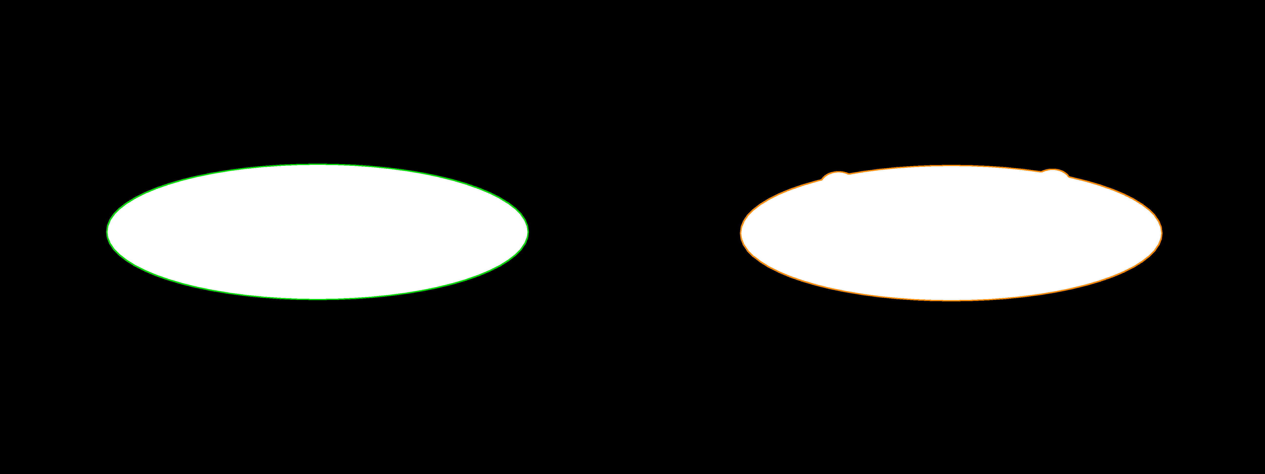
Figure 24.2 overlays the two contours back onto the original images: green for the master, orange for the test part. The subpixel point list hugs the centerline of the gray transition band, and the high-curvature ends of the ellipse are smooth and continuous — evidence that the backlit silhouette faithfully hands the crisp boundary to the subpixel extractor.

Figure 24.2: The extracted contours of the two parts. Left: the master (green, 3627 points); right: the top-defect part (orange, 3627 points). The backlit silhouette produces almost no stray contours, leaving one closed contour in each image.

24.2 Contour Features

A closed contour carries a full set of geometric quantities corresponding to the Blob features. Perimeter is the sum of adjacent point distances; area need not fill pixels and count them — Green’s theorem turns the region integral into a loop integral on the boundary (i.e. the shoelace formula), and the ordered point list gives the area directly. The center is the geometric midpoint of the bounding box, the gravity (centroid) is the centroid of the enclosed region, and the orientation comes from the principal axis of the second moments. Two dimensionless shape factors: circularity measures closeness to a circle (1 for a circle, smaller as the shape grows more elongated); rectangularity is the ratio of area to the smallest enclosing rectangle’s area. Measured values for the master contour:

Table 24.1: Measured features of the master contour (SciSvContourFeature)

Feature	Measured value
Area	751878.4 px²
Perimeter	3826.33 px
Center	(1300.53, 950.50)
Gravity	(1300.53, 950.52)
Orientation	−0.00°
Circularity	0.321
Rectangularity	0.785
Smallest enclosing rect	1726.7 × 555.0 @ −89.99°

This table is itself a self-check, and every number says “this is a standard ellipse”. The smallest enclosing rectangle is 1726.7 × 555.0 at orientation −89.99° — a major axis of 1726.7 px horizontal, a minor axis of 555 px vertical, a major-to-minor ratio of about 3.1. Rectangularity 751878.4/(1726.7×555.0) = 0.785, which is exactly \(\pi/4\): the ratio of an ellipse’s area \(\pi ab\) to its bounding-rectangle area \(4ab\) is precisely \(\pi/4≈0.785\) — a number clean enough to read off the geometric identity. Circularity 0.321 is low because this is a 3:1 flat ellipse, far from a circle. Most notably, the center and the gravity nearly coincide: (1300.53, 950.50) versus (1300.53, 950.52), differing by less than 0.02 px — the standard part’s outline is symmetric, so its centroid naturally lands at the geometric center; once a part carries an asymmetric defect, these two points separate, and the gap between center and gravity is itself a probe of shape asymmetry (the registration section below will use this point).

The definition of circularity varies among toolkits: some take \(4\pi A/P^2\), others \(A/(\pi r_{\max}^2)\) (with \(r_{\max}\) the maximum distance from center to contour). The two definitions give different values for the same shape, so comparing circularity across libraries is meaningless — being self-consistent within one production line is enough.

These features relate to Blob features (Chapter 23) as a “boundary version” to a “region version”: they ought to agree numerically, but the contour version is more accurate thanks to its subpixel point list and depends only on the boundary itself — when two targets touch into a single Blob on the region, their respective contours may still be cleanly separable. An honest note: the current SDK has no curvature API; when curvature is needed (e.g. to assess the corner quality of the ellipse ends), compute it yourself on the smoothed contour — the rate of change of the tangent angle of adjacent points divided by arc length (or a local circle fit on the point list) gives a discrete curvature estimate.

24.3 Contour Operations

Before measurement and comparison, one often needs three kinds of preprocessing operations on the contour.

Smoothing: a sliding-window average of the point coordinates. With a window of 31, the master contour’s perimeter shrinks from 3826.33 to 3820.25 (about 0.16%). The shrinkage is tiny, which precisely indicates that the backlit silhouette’s boundary is clean enough — there is little high-frequency jitter to filter. But the direction of the shrinkage is fixed: noise makes the point list jitter back and forth around the true boundary, the jittered serrations are all high-frequency components, and the perimeter, which accumulates point distances, counts the length of every serration; smoothing is low-pass filtering (replaying on a 1D point list what Chapter 6 does on an image), removing high-frequency jitter so the perimeter can only decrease. Engineering corollary: perimeter is systematically biased high by noise, so before measuring perimeter either smooth or fix the smoothing parameters to ensure comparability — under a clean silhouette this bias is small, but in a noisy image a fixed smoothing policy is the prerequisite for comparability.

Resampling: reduce the 3627 points to a specified count; the experiment resamples to a target of 300 points, obtaining 300 points approximately equidistant along the contour — to bound the cost of subsequent per-point computation, or to provide uniform samples for fitting. There is a parameter-semantics pitfall here, see Section 24.5.

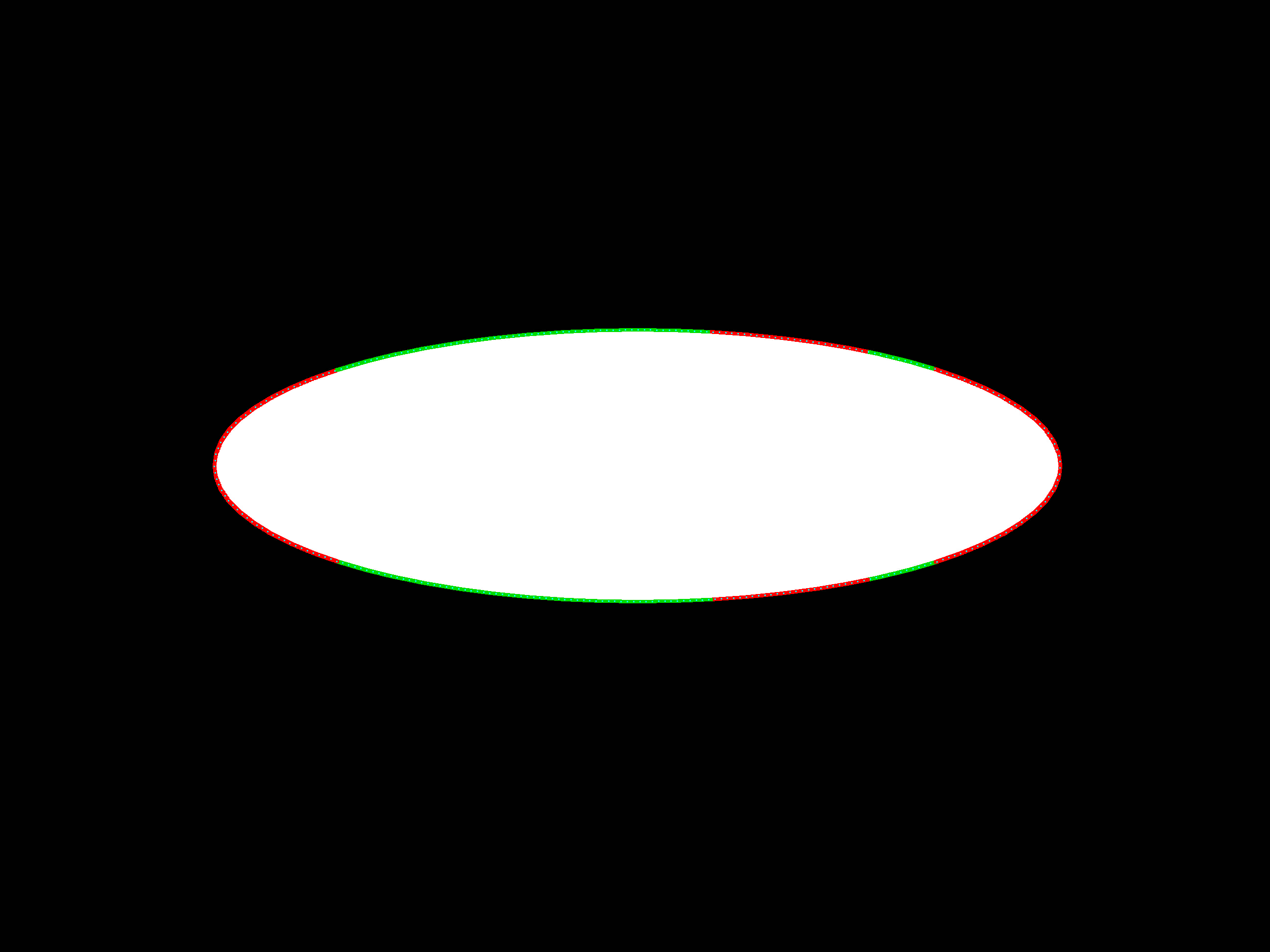
Segmentation: cut the contour into line segments and circular arcs by geometric property. The master contour splits into 16 segments = 12 lines + 4 arcs (Figure 24.3: line segments green, arc segments red, resample points as cyan ticks): the gentler arcs at the top and bottom of the ellipse are approximated by several short line segments (green), while the two high-curvature ends on the left and right are recognized as arcs (red) — this is exactly the sensible reading of “line-arc decomposition” for an ellipse: low-curvature regions as lines, high-curvature regions as arcs. The segment count and line/arc classification are sensitive to the smoothing amount and the two distance thresholds, so the parameters must be tuned to the feature size. The value of line-arc decomposition lies downstream: each line segment can be fitted for direction and position, each arc for center and radius, and the “contour” is upgraded into a dimensionable geometric drawing — paving the way for geometric measurement and robot path programming.

Figure 24.3: The result of operations on the master contour: after segmentation, line segments are green and arc segments are red (16 segments = 12 lines + 4 arcs, lines on the gentle regions and arcs on the high-curvature ends); the cyan ticks are the resampling to 300 approximately equidistant points.

24.4 Contour Comparison: Defect Detection

The climax of the chapter: compare the test part’s contour against the master’s point by point, letting positions where the deviation exceeds the tolerance surface automatically. The principle goes in three steps — registration: transform the master contour into the test part’s coordinate frame using a reference point and reference angle; per-point nearest distance: for each point of the test contour, find its nearest distance to the registered master contour; threshold decision: points whose deviation exceeds the tolerance maxDis are flagged as out of tolerance, and any out-of-tolerance point means NG. This is precisely the image-based inspection of the profile tolerance in GD&T: the actual contour is required to fall within a tolerance band of maxDis on each side of the theoretical contour.

The experiment uses maxDis=5 px. The registration basis comes from external localization: integrate the zeroth- and second-order moments of each image’s bright region to obtain its center and principal-axis angle (see below for why this is necessary). Comparing the top-defect part (003) against the master, the results:

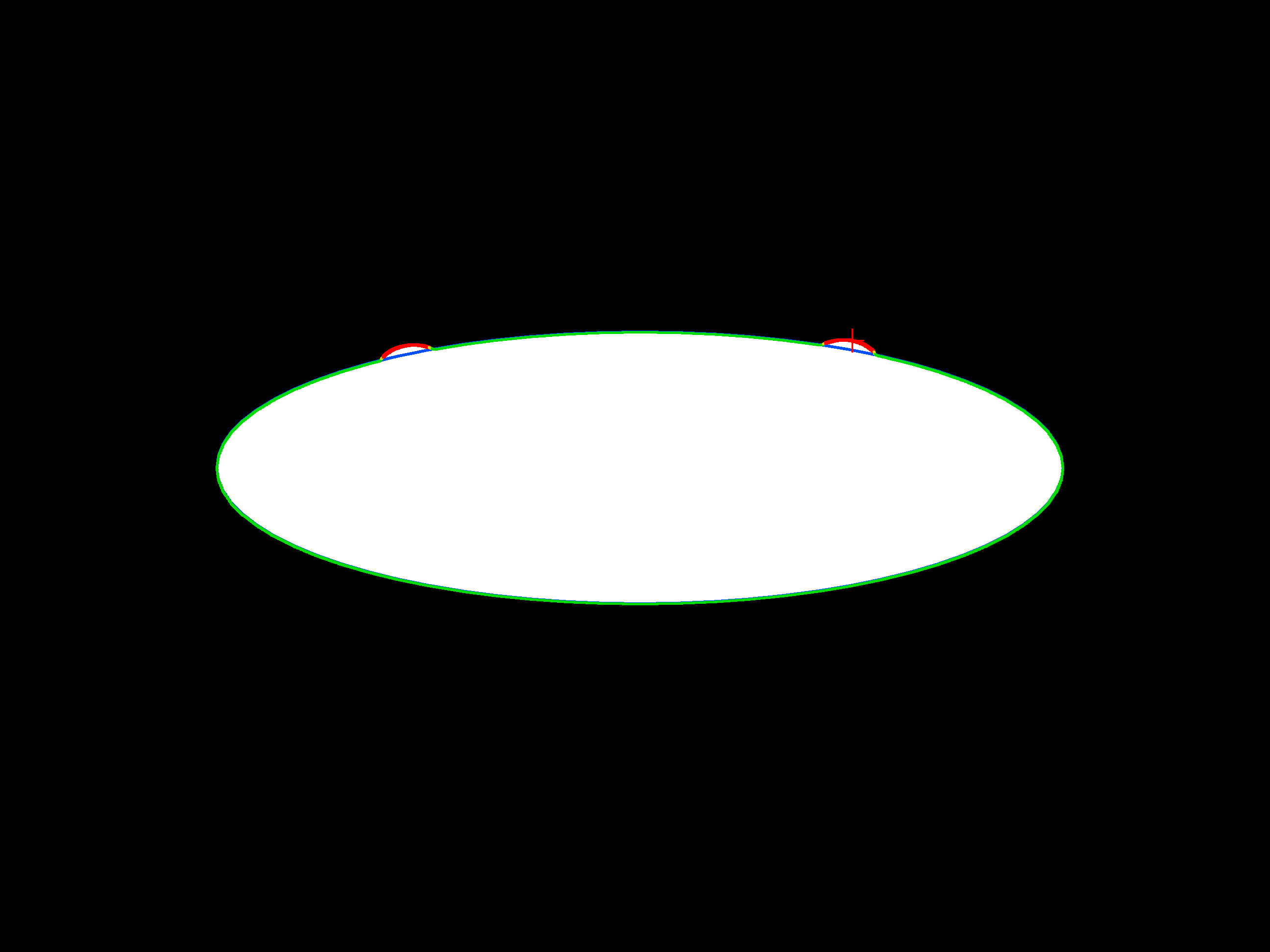
Maximum deviation 18.70 px @ (1738.5, 695.4) — the location is exactly the protrusion on the right of the top edge; the verdict is NG.
The per-point mean deviation is 1.64 px — this is the baseline fit of two independently imaged, independently registered subpixel contours over the full perimeter, about nine parts in ten thousand relative to the 1726.7 px major axis, the accuracy backbone of high-resolution silhouette extraction.
Two defect segments are localized automatically: segment #1 pts[418..514] (peak 18.70 px, the right protrusion on the top edge), segment #2 pts[3141..3232] (peak 17.86 px, the left protrusion on the top edge). GetOverThresholdContours likewise outputs 2 out-of-tolerance contour segments.
Switching to the bottom-bump part (002) against the master, the maximum deviation rises to 33.21 px @ (1554, 1250), mean 2.36 px, also NG — a larger bump yields a larger peak deviation.

Figure 24.4 rewards a color-by-color read: blue is the registered master contour — the “theoretical shape”; the test contour is colored by deviation, green ≤2 px, yellow 2–5 px, red >5 px; the red cross marks the maximum-deviation point. The two red clusters cover exactly the two protrusions on the top edge, and the rest of the contour is almost entirely green. Those two excess-material defects, which require a close look to discern by eye, have nowhere to hide on the deviation map — contour comparison turns “finding the defect” into “reading a thermometer”.

Figure 24.4: Contour comparison result. Blue: the registered master contour; the test contour is colored by deviation (green ≤2 px, yellow 2–5 px, red >5 px); the red cross is the maximum-deviation point at 18.70 px, located at the protrusion on the right of the top edge. The other protrusion on the left of the top edge is likewise captured by a red segment, two out-of-tolerance segments in all.

Per-point nearest distance is a one-directional measure: it only asks “how far is the test point from the master”, not the reverse. If the test part is missing a stretch of contour (e.g. a chip-out), the test points all still lie close to the master — a strict shape distance (such as the Hausdorff distance) takes the two-directional maximum. In practice one often runs the comparison once in each direction to cover both kinds of defect.

Finally, the most important lesson of this section: where does the registration reference point come from. First consider a naive assumption that the real sample images puncture directly — “all three images are the same workpiece, so the pose is of course the same, and an identity registration will do”. The measured external localization vetoes it: the master’s bright-region center is at (1300.00, 950.00), the top-defect part is at (1304.97, 954.02), off by 6.39 px, and the bottom-defect part is at (1301.25, 951.38), off by 1.86 px. Real capture has a positional drift each time the part is placed, so registration is not an identity transform and must be performed; forcing an identity registration would bake this 6.39 px global misalignment into every point and bury the defect signal entirely.

So what should the registration basis be? A seemingly handy approach is to use each contour’s own gravity — free to compute, the defect part using the defect part’s gravity. This chapter’s probe gives an honest comparison: the top-defect part’s contour gravity drifts 6.385 px relative to the master, almost exactly the 6.390 px measured by external localization — meaning the defect’s own contribution to the gravity is only about 0.005 px, and the two bases are nearly equivalent here (maximum deviation 18.697 versus 18.698 px). The reason is simple: the defect is too small relative to the whole large ellipse (the excess material is only parts per million of the bright region), the gravity displacement is dominated by the part’s real placement drift, and the defect cannot move it.

But the discipline still holds, and is proportional to the defect size: localizing the object by its own gravity is a systemic risk — the larger the defect, the more the excess (or missing) material drags the gravity off, the misalignment is read as a larger defect, and the measurement is contaminated by the measurand. Here the defect is small and the risk has not materialized; switch to a sample with a large burr and this path collapses. The robust approach is to take the reference point from external localization: a fixture, a locating pin, or moment integration / template matching on an uninspected region (the locating-datum problem discussed in Chapter 19 resurfaces here). This chapter uses moment integration over the entire bright region — which does two things at once: it corrects the 6.39 px real displacement, and, by covering a million pixels, it is naturally immune to local defects. The larger the defect, the more important this discipline.

24.5 SciVision Implementation

This chapter’s pipeline spans four classes. Extraction uses SciSvContourExtraction:

SCIMV::SciSvContourExtraction ext;
SciContourArray mAll;
long rc = ext.ExtractContours(srcM, fullROI, /*precision subpixel*/0, /*method canny*/1,
    /*filterCoeff*/2.0, /*lowThreshold*/20, /*highThreshold*/40,
    /*minContourLength*/600, /*maxContourLength*/100000, &mAll);

precision=0 outputs a subpixel contour; method=1 is the Canny route, filterCoeff is its smoothing scale, and the two thresholds are the hysteresis thresholds; minContourLength=600 is the filter threshold for stray contours. Note that maxContourLength has a valid range of [0, 100000] — passing a larger value (e.g. 1000000) raises a parameter error directly. Features use SciSvContourFeature, one call per feature:

SCIMV::SciSvContourFeature feat;
feat.GetContourArea(mC, &area);
feat.GetContourPerimeter(mC, &perim);
feat.GetContourCenter(mC, &center);
feat.GetGravityAndOrientation(mC, &gravity, &orient);
feat.GetContourCircularity(mC, &circ);
feat.GetContourRectangularity(mC, &rectg);
feat.GetSmallestRect(mC, &rcCenter, &rw, &rh, &rang);

Operations use SciSvContourOperation:

SCIMV::SciSvContourOperation op;
op.SmoothContours(mOne, /*window*/31, &smoothed);
op.SampleContour(mOne, /*method target point count*/1, /*sampleSize*/300.0, &sampled);
op.SegmentContours(mOne, /*smooth*/5, /*maxLineDistance1*/8.0f,
                   /*maxLineDistance2*/4.0f, &segs, &segType);

SegmentContours’s two distance thresholds control the allowed deviation of the line fit, and the output segType labels each segment’s type (0=line, 1=arc). Comparison uses SciSvContourContrast, with the reference point/angle coming from external localization (bright-region moments):

SCIMV::SciSvContourContrast cmp;
rc = cmp.ContrastContour(tOne, mOne, /*normRefPt*/refM, /*actRefPt*/refTest,
                         /*normAng*/angM, /*actAng*/angTest, /*maxDis*/5.0, /*outputMode*/0,
                         &maxPair, &maxOff, &results, &minPair, &minOff, &avgOff, &allOff);
SciContourArray overs;
cmp.GetOverThresholdContours(&overs);   // take the out-of-tolerance contour segments directly

There are two reference points/angles: norm* describes the master’s pose, act* describes the test part’s pose, and the registration transform is derived from their difference — here the two are measured independently from their own bright-region moments, thereby correcting the real placement drift. Pitfalls hit in practice (recorded in the engineering conventions):

Only outputMode=0’s scalar outputs are reliable. At outputMode=3, maxOff is a meaningless value (measured −0.052) and results misreads OK; the per-point allPointsOffset is complete in all modes (here 3627 signed deviations).
avgPointsOffset is unreliable: it returns 9.373 in measurement, whereas the true mean self-computed from allPointsOffset is 1.64 — compute the mean yourself.
SampleContour’s method=0/3 is upsampling, and only method=1 downsamples by target point count — pass 300 intending to reduce points and you may receive more points instead.
Some contour-related headers (SciSvContourOperation/ContourContrast etc.) unconditionally #define DLL_EXPORTS (an SDK slip); include them after the dllimport-style headers and they link normally.

The complete project that generates all the images and numbers in this chapter is in code/contour_analysis/, with the sample images in its sample/ subdirectory.

Industry Case: Seal-Ring Burr Inspection

After a rubber seal ring is vulcanized and demolded, the burr remaining at the parting line is the main defect, and a typical inspection scheme is exactly contour comparison: take a silhouette under backlight, extract the ring’s outer contour and compare it against a standard contour point by point, flagging out-of-tolerance as a burr — the same as the three ellipse samples of this chapter. One production line’s first version took a shortcut and used the part’s own gravity as the registration reference point — fine for small burrs (just as measured in this chapter, a small defect drags the gravity less than 0.01 px), but once a large burr appears, the excess material drags the gravity off, the registered standard contour shifts as a whole, and the intact edge on the opposite side is flagged out of tolerance over a large area, with “phantom defect” alarms firing frequently and re-inspection workload staying high. The revised scheme switched to the locating pin holes built into the mold as an external datum: locate the part’s pose by two pin holes first, then run the contour comparison, and the false-alarm rate immediately dropped to negligible. The lesson matches this chapter’s experiment exactly: the larger the defect, the less it can be allowed to take part in registration — the registration basis must be taken from external features unaffected by the defect.

24.6 Summary

A contour = an ordered string of subpixel boundary points, the “boundary-version dual” of the Blob region representation: the region suits statistics and connectivity, the contour suits boundary deviation, piecewise geometry, and high-precision measurement. The extraction pipeline is “edge detection → linking → subpixel refinement”, with the minLen length filter clearing stray contours; the backlit silhouette hands the crisp boundary to the subpixel extractor, and the three parts each yield a closed contour of 3627 points.
Contour features correspond one-to-one with Blob features but with higher accuracy: area is integrated directly from the boundary by Green’s theorem, rectangularity 0.785 is exactly \(\pi/4\) — self-proving this is a standard ellipse; the symmetric master’s center and gravity nearly coincide (differing <0.02 px), and the gap between the two is a probe of shape asymmetry. Shape factors such as circularity are defined differently across libraries and cannot be compared across libraries.
Smoothing is low-pass: a window of 31 takes the perimeter 3826.33→3820.25 — under a clean silhouette the shrinkage is only 0.16%, but its direction is fixed, so perimeter measurement must fix a smoothing policy; segmentation cuts the ellipse into 12 lines + 4 arcs (lines on the gentle regions, arcs on the ends), upgrading it into a dimensionable geometric description.
Contour comparison = registration + per-point nearest distance + tolerance decision, the image realization of profile-tolerance inspection: with a baseline deviation of 1.64 px, this chapter’s experiment cleanly captures the two protrusions on the top edge (peaks 18.70 and 17.86 px) and the bump on the bottom edge (peak 33.21 px), automatically localizing the defect segments and judging NG.
The registration basis is the make-or-break point: the three real-sample workpieces are not co-located (external localization measures offsets of 6.39 and 1.86 px), so registration must be performed and the basis must be robust — this chapter uses moment integration over the entire bright region to correct the real displacement and stay immune to local defects at once; using the part’s own gravity fails as the defect grows (here a small defect contributes only 0.005 px to the gravity, but a large burr would collapse it). Chapter 26 will generalize comparison-based defect detection to more general forms.

The classic algorithm for contour extraction (border following) is given by Suzuki and Abe (Suzuki and Abe 1985); the chain-code representation and processing of contours trace back to Freeman’s survey of computer processing of line-drawing images (Freeman 1974); and the polyline-simplification idea behind this chapter’s segmentation operation originates in the classic algorithm of Douglas and Peucker (Douglas and Peucker 1973). For a more systematic engineering treatment of subpixel contour extraction, contour segmentation, and contour-based measurement, see the work of Steger et al. (Steger, Ulrich, and Wiedemann 2018).