32 Structured Light 3D Imaging
The Achilles’ heel of binocular stereo vision (Chapter 31) is “finding correspondences”: the left and right images must be matched at the same physical points, and that matching relies on surface texture. Yet the industrial floor is full of texture-poor objects—polished metal surfaces, the uniform painted coats of injection-molded parts, white ceramics—on which every pixel looks identical, leaving the matching algorithm with nothing to grab onto and the disparity map riddled with large empty holes. If the object will not grow its own texture, then we project it on actively. This is exactly the core idea of structured light: a projector casts a set of known, controllable bright-and-dark patterns onto the object’s surface, making them serve as “artificial texture.” When the pattern lands on an undulating surface, it deforms with the height; the camera captures that deformation and inverts it to recover the height at every point. Among all the codable patterns, sinusoidal fringes + phase shifting is the workhorse of industrial 3D metrology—it encodes the height into the phase of the fringes, and phase can deliver subpixel, per-pixel dense reconstruction. Figure 32.1 shows the set of four-step phase-shifted fringes that runs through this entire chapter.
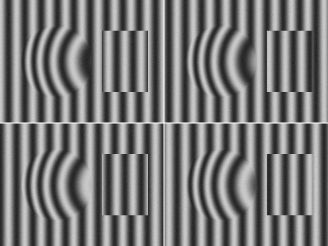
Why sinusoidal fringes rather than binary Gray code? Gray code encodes only “black/white” per pixel, so its resolution is limited by the finest line width of the fringes; the sinusoidal phase is a continuous quantity, and combined with phase shifting it can resolve the fractional phase inside a pixel, raising accuracy by one or two orders of magnitude. The price is that the phase has a \(2\pi\) periodic ambiguity that must be unwrapped—precisely the problem Section 32.2 of this chapter sets out to solve.
32.1 Principle of Phase Shifting
Suppose the projector casts spatial sinusoidal fringes; the gray value the camera samples at pixel \((x,y)\) can be written as
\[ I_k(x,y) = A(x,y) + B(x,y)\cos\!\big(\varphi(x,y) + k\,\tfrac{\pi}{2}\big), \qquad k=0,1,2,3. \]
Here \(A\) is the background light (the DC component), \(B\) is the fringe modulation, i.e. the amplitude of the sinusoid, and \(\varphi\) is the phase we are really after—it encodes the height at that point. We project four fringe images in succession, each shifting the initial phase as a whole by \(\pi/2\) (this is “four-step phase shifting”), so the same pixel yields four equations, and the unknowns are exactly the three quantities \(A\), \(B\), and \(\varphi\). Subtracting the four equations pairwise:
\[ I_3 - I_1 = 2B\sin\varphi, \qquad I_0 - I_2 = 2B\cos\varphi. \]
Dividing and taking the arctangent, \(A\) and \(B\) are eliminated together, leaving only the phase:
\[ \varphi(x,y) = \operatorname{atan2}\big(I_3 - I_1,\; I_0 - I_2\big). \]
This formula is the whole essence of phase shifting. What is worth savoring repeatedly is the source of its robustness: \(\varphi\) depends only on the differences and ratio of the four intensities, and is independent of the background light \(A\) and of the fringe brightness \(B\). In other words, camera gain drift, ambient-light fluctuation, and the high or low albedo of the measured surface none of them change the recovered phase—they alter only \(A\) and \(B\), and both of those have already been eliminated. This is the same engineering wisdom as the “gradient direction does not change with illumination gain” of Chapter 17: encode the information into a quantity that is invariant to gain, and the measurement becomes stable. Intensity itself is fragile; phase is reliable.
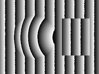
The range of \(\operatorname{atan2}\) is \([-\pi,\pi)\), so the recovered phase is the wrapped phase—every time the true phase exceeds a \(2\pi\), it is folded back into this interval, forming a sawtooth. Figure 32.2 illustrates this: a continuously undulating height field turns into bands of equal phase in the wrapped-phase image, with “cliffs” plunging from \(+\pi\) down to \(-\pi\) between the bands. These cliffs are not real discontinuities but artifacts of the periodicity of \(\operatorname{atan2}\); the next section will smooth them out.
32.2 Phase Unwrapping
To restore the wrapped phase \(\varphi\in[-\pi,\pi)\) to the continuous absolute phase \(\Phi = \varphi + 2\pi n\), one must determine the integer fringe order \(n\) pixel by pixel. The most naive approach is spatial unwrapping: scan along the image, and whenever the phase difference between adjacent pixels suddenly jumps past \(\pi\), judge that a wrapping cliff has been crossed and add a \(2\pi\) to all subsequent pixels. It works on smooth, connected surfaces, but it is disturbingly fragile—the moment it meets a false jump caused by noise, or a real height discontinuity on the object (such as the step in this chapter), the integration goes wrong by one or more whole \(2\pi\) from some point onward, and the error propagates all the way along the scan direction with no way to self-heal.
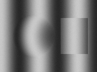
More robust in industry is the dual-/multi-frequency hierarchical method (dual-/multi-frequency unwrapping). Its idea is to use two sets of fringes with different periods: one low-frequency set with a period large enough that the phase varies by less than \(2\pi\) across the entire field of view, so it is naturally unambiguous and can directly tell us “roughly which fringe we are on”; and another high-frequency set with a small period and a steep phase slope, providing the final measurement accuracy. Figure 32.3 is the low-frequency set used in this chapter (\(P=128\) px, four times the high-frequency \(P=32\)). Specifically, we first perform one spatial unwrapping of the low-frequency wrapped phase to obtain the low-frequency absolute phase \(\Phi_{\text{lo}}\) (the low-frequency field is smooth, the phase jump caused by the step is only about \(0.6\) rad, far less than \(\pi\), so the spatial unwrapping will not go wrong), then use the frequency ratio \(P_{\text{lo}}/P_{\text{hi}}=4\) to scale it up and predict the high-frequency absolute phase, rounding to fix the order pixel by pixel:
\[ \Phi_{\text{hi}} = \varphi_{\text{hi}} + 2\pi\,\operatorname{round}\!\Big(\frac{\Phi_{\text{lo}}\cdot(P_{\text{lo}}/P_{\text{hi}}) - \varphi_{\text{hi}}}{2\pi}\Big). \]
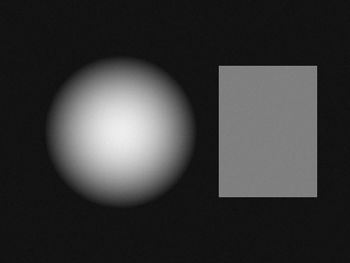
The key point is this: the order \(n\) is computed independently per pixel, without relying on neighborhood integration, so an error at one pixel can never infect its neighbors—the real discontinuity of the step is preserved faithfully, rather than being “smoothed away.” This is the fundamental reason the dual-frequency method dominates the spatial method. Figure 32.4 is the absolute phase after unwrapping: smooth and monotone, with the dome of the spherical cap and the block of the step clearly distinguishable.

Unwrapping has another technical route: temporal phase unwrapping. Instead of looking for cliffs in the spatial neighborhood, it projects, onto the same pixel, several sets of fringes of increasing frequency over time, using the absolute phase of the previous frequency to assign the order for the next. The dual-frequency method is its most stripped-down two-level special case. The temporal method’s advantage is that it is point-independent and discontinuity-resistant; its drawback is that the number of projected frames doubles, making it unsuitable for high-speed motion scenes—the classic speed-versus-robustness trade-off.
32.3 Height Reconstruction and Accuracy
The final leap from absolute phase to height is a triangulation calibration relation. In this chapter’s imaging model, the projector coordinate \(u = x + c\cdot h\), where \(h\) is the height and \(c\) is the triangulation constant determined by the projector–camera geometry (here \(c=4\) px/mm, i.e. 1 mm of height shifts the fringe laterally by 4 px). The relation between the absolute phase and the projector coordinate is \(\Phi = 2\pi u / P_{\text{hi}}\), and solving the two together inverts to:
\[ h(x,y) = \frac{1}{c}\Big(\frac{\Phi_{\text{hi}}\,P_{\text{hi}}}{2\pi} - x\Big). \]
The measured accuracy is satisfying. Under the conditions \(A=120\), \(B=80\), noise \(\sigma=3\), the apex of the spherical cap reconstructs to 5.994 mm, against a ground truth of 5.994 mm; the step height is 2.999 mm, against a ground truth of 3.000 mm—both hit the mark. Figure 32.5 is the final height map. The RMS noise floor on the flat base plane is 0.0338 mm, and that is the height repeatability of this configuration.
Where does this noise floor come from, and what determines it? The answer is the lifeblood of structured light—the modulation \(B\). Propagating the error through four-step phase shifting, the standard deviation of the phase satisfies
\[ \sigma_\varphi \approx \frac{\sigma}{B}, \]
that is, the phase noise is inversely proportional to the fringe amplitude. Drop \(B\) from 80 to 15 (about \(5.3\times\)), and in theory the phase and height noise should be amplified by the same factor. Experiment shows: at \(B=15\) the base-plane RMS rises to 0.1823 mm, exactly 5.4 times the 0.0338 mm at \(B=80\)—almost perfectly matching the 5.3-fold theoretical prediction. This \(\sigma_\varphi\propto\sigma/B\) law translates an abstract image-quality metric (how clear the fringes are) directly into height accuracy. The accuracy of structured light is, in essence, determined by the modulation. Every factor that suppresses \(B\)—dark surfaces, low-contrast projection, defocus, motion blur—degrades the 3D accuracy proportionally.
\(\sigma_\varphi\approx\sigma/B\) also explains why industrial structured-light systems strive to project high-contrast fringes: projector brightness, lens aperture, camera exposure—they all ultimately serve one goal, pushing \(B\) to its maximum without saturating. But the premise “without saturating” is crucial; the next section will show that once the line is crossed, catastrophe arrives in another form.
32.4 Modulation, Saturation, and Surfaces
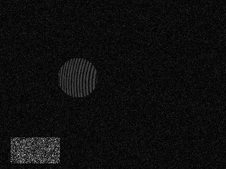
Since \(B\) determines accuracy, a natural engineering move is to use a modulation mask to reject pixels whose \(B\) is too low—four-step phase shifting incidentally computes \(B=\tfrac12\sqrt{(I_3-I_1)^2+(I_0-I_2)^2}\), and thresholding it does the job. In this chapter’s “real-capture” experiment, a dark region with an albedo of only 0.18 is embedded in the lower-left corner of the base plane, simulating black paint or a low-reflectance surface. The result is beautiful: with \(B<20\) as the threshold, 99.7% of the dark-region pixels are flagged, while the clean base plane has zero false alarms—the mask precisely circles out the untrustworthy region. The left of Figure 32.6 is the modulation map, the right is the binary mask.

But the modulation mask has one fatal blind spot: it cannot block saturation. The experiment overlays a specular highlight on top of the spherical cap (clipped at 255 after a 1.7× gain), simulating a metallic reflection. Intuitively, saturation would destroy the sinusoid and lower the modulation, so the mask ought to catch it—but the measured fraction of the saturated region that is flagged is 0%. The reason is this: the four phase-shifted images are clipped equally to 255, and the differences \(I_3-I_1\) and \(I_0-I_2\) still retain a fair amount of amplitude after clipping, so the computed \(B\) does not drop below the threshold. The mask therefore believes the region has “good modulation, trustworthy data,” when in fact the phase has already been distorted by clipping. The consequence is that the apex of the spherical cap shifts from 5.994 mm to 5.928 mm, the RMS inside the saturated disk rises to 0.1087 mm (about 3.2 times the clean region), and the dark-region RMS is 0.1911 mm. The mask fails, and only the error map can expose the truth—Figure 32.7 plots the reconstruction error, and the error gathers into exactly two clusters: the dark region and that saturated highlight disk, precisely coinciding with the locations the mask missed.
This puts on the table the “compatibility” of different surfaces with structured light. Dark/low-albedo surfaces suppress \(B\) and amplify noise, and can be rejected by the mask; saturated highlights quietly inject a systematic bias right under the mask’s nose and must be prevented at the source by exposure control (avoiding crossing the line; echoing the illumination design of Chapter 4); translucency and subsurface scattering make the fringes “bleed” and distort the phase. There is also a class of surfaces structured light simply cannot handle—mirrors: the light is reflected away by the mirror surface, and the camera never receives the fringes landing on the surface; here one must switch to deflectometry (Chapter 35), which measures not the fringe position but the deflection of the pattern by the surface normal. No single 3D method works on every surface; the boundary of structured light is precisely the boundary of its method assumptions (Chapter 30).
32.5 SciVision Implementation
This chapter originally planned to reuse the SDK’s phase-measurement module SCIMV::SciSvPhaseMeasure, but its core entry points proved unusable in testing, faithfully recorded here. DecodePatterns (four-step phase-shift decoding), under all 16 call variants we tried—8U and 32F input, with and without a prior InitPMD, UNDEF and full-image rectangular ROI, with and without a supplementary set of Y-direction fringes—all returned rc=0 yet produced no output whatsoever: the phase map, gray map, and modulation map were all \(0\times0\) empty objects, and the DLL even printed a “Directory does not exist.” to stderr (apparently a missing runtime resource directory). CalUnPhase (spatial unwrapping), which depends on its output, was consequently unusable as well. The entire pipeline is therefore written entirely by hand. There are only two core snippets, but they are the whole of this chapter’s algorithm:
// 1. Four-step phase-shift wrapped phase + modulation (A, B cancel in the differences, leaving only the phase)
for (size_t i = 0; i < (size_t)W * H; ++i) {
    double s = (double)im[3][i] - im[1][i];   // =  2B*sin(phi)
    double c = (double)im[0][i] - im[2][i];   // =  2B*cos(phi)
    phi[i] = std::atan2(s, c);                // wrapped phase [-pi, pi)
    mod[i] = 0.5 * std::sqrt(s * s + c * c);   // modulation ~ B
}

// 2. Dual-frequency hierarchical unwrapping: low-freq absolute phase *4 predicts high-freq order, rounded per pixel (no neighborhood integration)
const double ratio = P_LO / P_HI;             // 128/32 = 4
for (size_t i = 0; i < abs.size(); ++i)
    abs[i] = wHi[i] + TWO_PI * std::round((uLo[i] * ratio - wHi[i]) / TWO_PI);
The first snippet directly implements the arctangent formula of Section 32.1: im[k] is the \(k\)-th phase-shifted image, s and c are proportional to \(\sin\varphi\) and \(\cos\varphi\) respectively, atan2 gives the wrapped phase, and the modulation is obtained incidentally from the magnitude of the two. The second snippet is the hierarchical method of Section 32.2: uLo is the spatially unwrapped low-frequency absolute phase, which after multiplying by the frequency ratio 4 predicts the high-frequency absolute phase, and std::round assigns each pixel independently to the nearest integer multiple of \(2\pi\). The complete runnable project is at code/structured_light/, including fringe synthesis, the low-modulation rerun, and the real-capture trap experiments.
Industry Case: Reflective Solder and Black Ink in SPI
PCB solder-paste printing inspection (SPI, Solder Paste Inspection) is a classic battlefield for structured-light 3D—it must measure the volume of every blob of solder paste point by point, directly bearing on the soldering yield. The difficulty is exactly this chapter’s dilemma in one frame: the freshly printed solder paste has a metallic luster and is highly prone to specular reflection and saturation; the black solder-mask ink beside it has extremely low albedo and all but swallows the light. Tune the exposure for the solder paste, and the black-ink region’s phase drowns in noise; tune it for the black ink, and the solder-paste highlights saturate and inject a systematic height bias—and saturation, in turn, fools the modulation mask, so the bias creeps in silently.
The practical countermeasure is HDR multi-exposure fused fringes (echoing Chapter 12): for each phase-shift phase, project several exposure levels, and per pixel pick the level that is unsaturated and has the highest modulation to fuse, letting the solder paste and the black ink each take what they need. The lesson is plain yet profound: the whole-field accuracy of structured light is determined by the worst modulation anywhere in the field—optimization must target the weakest surface, not the average one.
32.6 Summary
- No texture? Project it on. Binocular stereo relies on surface texture to find correspondences, and smooth objects make it fail; structured light projects a controllable “artificial texture,” encoding height into the fringe phase to achieve dense 3D reconstruction.
- Phase is more robust than intensity. Four-step phase shifting \(\varphi=\operatorname{atan2}(I_3-I_1,\,I_0-I_2)\) eliminates both the background light \(A\) and the fringe amplitude \(B\), making the phase insensitive to gain, ambient light, and albedo—this is the foundation of stable measurement.
- Wrapping must be undone; dual-frequency is the most robust. The \(2\pi\) ambiguity of \(\operatorname{atan2}\) must be removed by unwrapping; the spatial method integrates point by point and collapses at discontinuities, while the dual-/multi-frequency hierarchical method assigns orders per pixel and resists discontinuities, and is the industry standard.
- Modulation is the lifeblood. The height noise \(\sigma_\varphi\propto\sigma/B\); measured, \(B\) dropping 5.3× raised the error 5.4×; every factor that suppresses \(B\) degrades accuracy proportionally.
- The mask cannot block saturation. The modulation mask can precisely reject the dark region (99.7%, zero false alarms), yet is blind to saturation (0% flagged)—saturation does not lower the modulation but distorts the phase, and only the error map can expose it; defending against saturation relies on exposure control and HDR, not an after-the-fact mask.
For a systematic taxonomy of structured-light coding patterns, see the survey by Salvi et al. (Salvi et al. 2010); the development and key issues of fringe-projection profilometry are reviewed by Gorthi and Rastogi (Gorthi and Rastogi 2010), while Geng’s tutorial (Geng 2011) gives a systematic and accessible overview of the various structured-light 3D-imaging methods. Implementation details of phase-shift profilometry and multi-frequency unwrapping in industry can be further consulted in the book by Steger et al. (Steger, Ulrich, and Wiedemann 2018).