18 Feature and Color Matching
The matching methods of the previous two chapters share one trait: they are all dense — gray-value matching (Chapter 16) compares an entire template pixel by pixel, shape matching (Chapter 17) compares an entire contour point by point, and pose (angle, scale) must be searched as explicit dimensions step by step, with cost growing as the range widens. This chapter introduces two kinds of matching that take a different road altogether. Feature matching compresses an image into a few dozen keypoints; what gets compared is no longer a patch of pixels but a sparse point set — when a part may appear at an arbitrary angle, or even at a different scale, its cost barely grows with the pose range. Color matching abandons geometry entirely: in a sorting task like “is this a red cap or a yellow cap,” what matters is not where the part is or how far it has rotated, but what color it is — classifying by color statistics is more direct than any geometric matching.
The feature-matching part uses a set of real industrial sample images: the sample sheets from Smart3’s “feature matching” locating recipe — a five-armed rotor/sprocket casting, imaged under dark-field illumination as \(1000\times 800\) 8-bit grayscale. The same physical part appears in four images at different positions and angles, which is exactly where feature matching shines. We crop a part-sized square out of one of them (rotor_001, the part roughly centered and high) to use as the template (Figure 18.1 (a)), and search for it in the other three (rotor_002/003/004). The part’s surface is covered with sandblast casting texture and dotted with through-holes, slots, and arm tips, so corners abound; yet it is also near five-fold rotationally symmetric — which plants a real pitfall for matching, detailed below. The color-matching part keeps synthetic data: this “feature matching” sample set is single-channel grayscale and cannot drive color matching, so to fully present the use and chromatic behavior of SciSvColorMatch, the color experiment uses a synthetic red/green/blue/yellow bottle-cap sorting scene, as noted in Section 18.4.
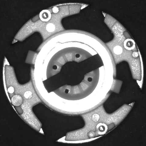
rotor_001 (\(480\times 480\))
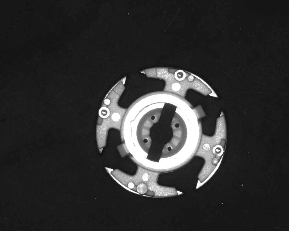
rotor_002, the part in another pose
rotor_001 — the sandblast texture, through-holes, slots, and five arm tips provide hundreds of corners; (b) one \(1000\times 800\) search image: the same part on a dark field at a different position and rotation, the background near-black and featureless.
18.1 Keypoints and Descriptors
The first step of feature matching is to pick out a small number of “distinctive” points from the image. What makes a point distinctive? A pixel inside a flat region looks the same wherever its neighborhood is shifted — there is nothing to recognize; a point on an edge keeps a nearly unchanged neighborhood while sliding along the edge, so only one direction can be pinned down. Only a corner — a point where the gray value changes sharply along two independent directions — has a neighborhood that differs under every translation and can be uniquely “recognized.” This is the same intuition as corners serving as salient contour points in Chapter 25: the detector scans the image for locations where the local “cornerness” is strongest and exceeds a threshold, and takes those as keypoints.
Position alone is not enough — we must also be able to recognize the same point in another image. For this, a descriptor is computed over each keypoint’s neighborhood: the gray-value or gradient distribution of the neighborhood is encoded into a feature vector that serves as the point’s “fingerprint.” The point pairs whose descriptors are closest across the two images become candidate correspondences. For the same corner to keep a similar fingerprint after rotation, the descriptor first estimates the dominant orientation of the neighborhood and rotates the neighborhood into a canonical orientation before encoding — this is where rotation invariance comes from: the angle is not found by exhaustive search but is “digested” by the descriptor.
This is precisely where sparse matching turns the cost tables. Dense template matching must traverse the pose space: a grid of position \(\times\) angle \(\times\) scale, with a full-template comparison at every grid point — double the angle range and the cost doubles. Feature matching splits the pipeline into three steps: detect keypoints (once per image, independent of pose), compare a few dozen descriptors, and finally solve for the pose from the candidate correspondences — the pose space is never enumerated from start to finish. The candidate correspondences inevitably contain misrecognized outliers, so the pose is solved with RANSAC: repeatedly draw a minimal point set at random, fit a rigid (or similarity) transform, and count how many correspondences agree with that transform — the inliers; the transform with the most inliers wins, and the pose is refined by least squares over all inliers.
We already used RANSAC when fitting lines in Chapter 14: amid data contaminated by outliers, “draw minimal samples at random, vote for a consensus” is far more robust than least squares. There the outliers were stray edge points; here they are misrecognized descriptor correspondences — the recipe is exactly the same.
A quick cost ledger: covering \(360^\circ\) on this chapter’s samples with gray-value matching at a \(1^\circ\) step would require preparing 360 template poses and scanning each one; feature matching only detects keypoints once (about 410 per search image here), then finds correspondences among descriptor pairs on the order of \(335\times{\sim}410\) — and however much wider the angle range gets, this bill does not change.
There is no free lunch, of course: feature matching requires the template to have enough detectable corners. A smooth, textureless part (a disk, a plain plate) yields hardly any keypoints, and the model simply cannot be built — this chapter’s rotor casting is the opposite case, with corners everywhere across its sandblast surface and its holes, slots, and arm tips, a “friendly” subject for feature matching. But it brings a different, very real trouble: near five-fold rotational symmetry. On a geometrically self-similar part, descriptors on different arms look alike, and the pose can easily settle on a “displaced” consensus — exactly the engineering pitfall the next section confronts.
18.2 Feature Matching Experiment
The template comes from rotor_001: we first threshold the part by brightness to find its centroid (\((533.3,492.6)\)) and crop a \(480\times 480\) square around it (Figure 18.1 (a)). Training on the template with the STABLE detector yields 335 model feature points (Figure 18.2): they blanket the sandblast surface, the through-hole and slot edges, and the arm tips — the places of strongest cornerness. The same model finds about 410 scene keypoints in each of the three \(1000\times 800\) search images (420 / 414 / 406).
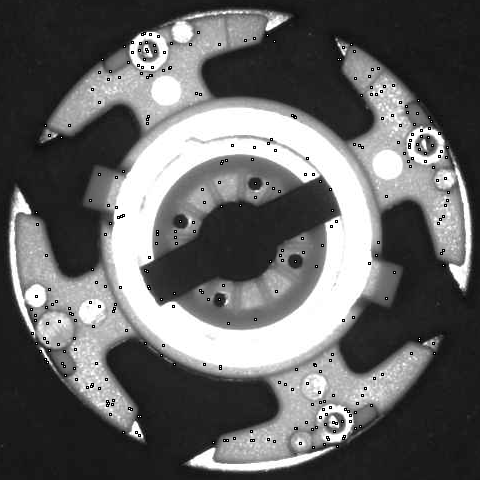
The real samples carry no ground-truth pose, so we validate the matches with two mutually independent lines of evidence. The first is a known-answer self-match: searching for the model back in its own source image rotor_001 should return it to the template origin. The measured location is \((533.00,493.00)\), angle \(0.000^\circ\), scale \(1.0000\) — an error of 0.00 px against the template origin \((533,493)\), which zeroes out the entire crop-model-search chain. The second is a cross-check against the intensity centroid: the rotor is nearly centrally symmetric, so its brightness centroid is a stable physical reference entirely unrelated to feature matching; if the solved center agrees with it, the two corroborate each other.
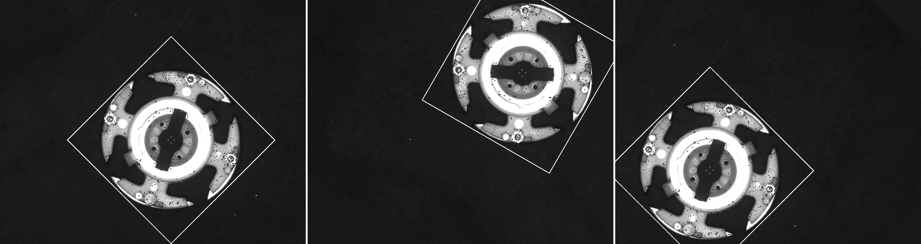
The matching results for the three images (Figure 18.3) are clean, every one hitting on the first try at the strictest matcher threshold, 60:
| Search image | Solved center | Angle | Scale | Intensity centroid | Center error |
|---|---|---|---|---|---|
rotor_002 |
\((558.72,458.24)\) | \(-44.97^\circ\) | \(0.9996\) | \((558.6,457.8)\) | 0.43 px |
rotor_003 |
\((701.58,239.17)\) | \(-149.99^\circ\) | \(0.9995\) | \((701.1,239.4)\) | 0.51 px |
rotor_004 |
\((308.59,558.20)\) | \(-44.98^\circ\) | \(1.0000\) | \((308.6,557.8)\) | 0.37 px |
The center errors are all on the order of 0.5 px, and the scales without exception fall within \(0.05\%\) of \(1.000\) — squarely consistent with the physical fact of “same camera, same working distance, unscaled part,” strong corroborating evidence that the results are sound. Note that we never told the matcher the angle range: rotations from \(-45^\circ\) to \(-150^\circ\) were absorbed naturally by the descriptors and RANSAC. And one subtle but important point: the solved angles (\(-45^\circ\), \(-150^\circ\)) are not integer multiples of the five-fold symmetry step \(72^\circ\) — which means the match was not “talked into” some symmetry-equivalent solution by the rotational symmetry, but anchored a genuine absolute orientation through the casting’s unique sandblast texture.
This experiment exposed an engineering reality textbooks almost never write down but that is enough to wreck a deployment on the line: the choice of descriptor. The first attempt used the STABLE detector plus the STABLE descriptor (the manual’s “robust” default pairing); the self-match was perfect and rotor_003 localized to 3.6 px, but rotor_002 and rotor_004 were both badly displaced — centers off by 183 px and 52 px, scales drifting to \(1.06\) and \(0.78\), and the matcher threshold having to be relaxed all the way to 10 before any result appeared. The root cause is exactly the near five-fold symmetry planted in the previous section: the STABLE descriptor lacks the discriminating power to tell the self-similar arms apart, and RANSAC voted its consensus onto a rotation-displaced solution. Switching to the FAST descriptor made all three images hit at the strict threshold 60, with center errors down to 0.5 px and scales back at \(1.00\) — same detector, same set of keypoints, only the descriptor changed, and the results were worlds apart. The lesson: on geometrically self-similar parts, the descriptor’s discriminating power matters more than the detector’s point count; “default parameters” are not necessarily tuned for your part, and a quick empirical sweep over the competing parameters often finds the answer faster than reading the manual.
One more SDK semantic is worth recording: even with matchCount set to 2, FindFeatureImageModel returns only 1 instance per call — RANSAC picks the single transform with the most inliers, and in its eyes the second-best instance’s correspondences are just a pile of outliers. Each image here happens to contain exactly one part, so one call per image suffices; but if an image held several copies of the same part, the application layer must iterate “find one → erase it from the image → find again.”
Finally, the source of sparse matching’s robustness deserves a word: the model points in Figure 18.3 map precisely onto each part because the pose is determined by the geometric consistency of the point group, not the accuracy of any single point. The detector only recognizes “cornerness,” so individual candidate correspondences inevitably connect to the wrong arm or to a bright background speck; what rules them out is the hard constraint that all 335 model points must fall into place at once. The robustness of sparse matching lies not in the accuracy of any single point, but in the agreement of the group.
18.3 Representing and Matching Color
Switch scenes: red, green, blue, and yellow bottle caps stream past on a conveyor, and the task is to sort them. Geometry is completely irrelevant here — the caps are all round — what matters is only the color. The most naive approach treats a region’s mean color as a three-dimensional vector \((R,G,B)\), computes the Euclidean distance to each reference color, and lets the nearest one win.
There is a mine buried in this approach: RGB couples brightness and chromaticity together. Take the same red cap and dim the lighting by thirty percent — the three components of \((R,G,B)\) shrink in nearly equal proportion, the color vector slides along the ray toward the origin, and its Euclidean distance to the reference color grows, even though to the human eye it is “still that same red.” On a production line, lamp tubes age, voltage fluctuates, and workpieces sit at varying distances from the lights — brightness is never a constant; sorting by raw RGB distance amounts to betting the classification threshold on the stability of the illumination.
The fix is to divide the brightness out of the color, keeping only the “ratio of the colors” — this is chromaticity. The simplest chromaticity coordinates are normalized RGB:
\[ r = \frac{R}{R+G+B}, \qquad g = \frac{G}{R+G+B}, \]
(with \(b\) given by \(r+g+b=1\)). Multiply all three components by a common gain and the numerator and denominator scale together — \((r,g)\) does not budge. A linear brightness change is canceled exactly, the same idea by which NCC cancels the illumination gain through normalization (Chapter 16), replayed in color space. The separation of hue H, saturation S, and value V in HSV space (already used for color thresholding in Chapter 7) is another realization of the same idea, with equivalent engineering effect.
The geometric picture: in RGB space, points of “same color, different brightness” line up on a ray through the origin; chromaticity normalization projects each ray onto a single point on the plane \(R+G+B=\text{const}\). Classification is done on this plane, with the brightness dimension folded away entirely.
The color matcher is used one model per class: train one color model for each reference color, score the region under test with every model, and the highest score gives the predicted class. Whether its internal color representation is chromaticity-like is something the manual may never say outright — but we can interrogate it with an experiment.
18.4 Color Matching Experiment
This section uses synthetic data: the Smart3 samples used for feature matching above are single-channel grayscale and cannot carry color information, so to fully demonstrate the use of SciSvColorMatch and probe its internal color representation, we construct a color-patch sorting scene. The reference samples are four bottle-cap color patches (red/green/blue/yellow, each with \(\pm 10\) uniform noise added per pixel per channel, Figure 18.4). The test set is a \(3\times 4\) grid (Figure 18.5): the four columns correspond to the four colors, and the three rows multiply the caps’ brightness by \(0.8\times\), \(1.0\times\), and \(1.2\times\) respectively — simulating \(\pm 20\%\) fluctuations in illuminance and reflectance.

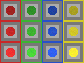
The classification result is clean: 12/12 correct, with true-class scores falling between 81.7 and 92.9 and an average margin over the strongest wrong class of about 40 points — not a narrow win but a rout.
The real point of this experiment, however, is not the accuracy but the brightness sweep. Averaging the true-class scores by row:
| Brightness | \(0.8\times\) | \(1.0\times\) | \(1.2\times\) |
|---|---|---|---|
| Mean true-class score | 91.0 | 89.9 | 84.1 |
With brightness swinging \(20\%\) up and down, the score curve is nearly flat — a maximum drop of only 5.8 points. If the matcher used raw RGB distance internally, a \(\pm 20\%\) brightness change would push the color vector quite far from the reference, and the score should slide substantially; the flat curve points to a different conclusion: this SDK’s color matching behaves close to a chromaticity space, not raw RGB distance. The slight dip in the \(1.2\times\) row also has a sound explanation: the yellow cap’s R-channel reference value is 210; multiplied by \(1.2\) it reaches 252, already brushing the ceiling of 255, and with \(\pm 10\) noise added it gets clipped — saturation genuinely shifts the chromaticity, so the points docked are docked for good reason.
One methodological detail deserves to be spelled out. We also ran two hand-written baselines: classification by raw RGB distance on the disk means, and by chromaticity distance — both also scored 12/12. This tells us the four-color sorting task is simply too easy: red, green, blue, and yellow sit far apart in hue, and \(\pm 20\%\) brightness is not enough to make raw RGB stumble, so accuracy as a metric has zero discriminating power on the question “is the SDK chromaticity-based.” What can separate the two hypotheses is the shape of the score curve: the raw-RGB hypothesis predicts scores sliding visibly with brightness, the chromaticity hypothesis predicts a flat curve — and the measurements side with the latter. When designing an experiment, make the competing explanations issue different predictions; otherwise even the prettiest numbers are mere self-congratulation.
18.5 SciVision Implementation
Feature matching is handled by SCIMV::SciSvFeatureMatch, in two steps — training and search:
SCIMV::SciSvFeatureMatch fm;
SciROI mask; // default-constructed = UNDEF, meaning the whole image (it must be!)
SciMatchModel model;
fm.CreateFeatureImageModel(tmplImg, mask,
SCI_FEATUREMATCH_DETECTOR_STABLE, // detectorMethod: 0=STABLE 1=FAST 2=EDGEPOINT
SCI_FEATUREMATCH_DESCRIPTOR_FAST, // descriptorMethod: FAST far beats STABLE on this part
/*sampleStep*/ 1, // sampling step: 1/2/4 — larger means sparser points, faster
/*scaleRange*/ 0, // scale levels 0..3, 0 = no scale expansion
/*detectorThreshold*/ 30, // corner-response threshold [1,255]; higher means fewer points
&model);
SciFeaturePointArray pts;
fm.GetFeatureModelPoints(model, &pts); // 335 model feature points in this example
SciPointArray centers; SciVarArray angles, scales;
fm.FindFeatureImageModel(sceneImg, roi, model,
SCI_FEATUREMATCH_MATCHER_STABLE,
/*matcherThreshold*/ 60, // match-quality floor [1,100]; the strict 60 hits all three here
/*matchCount*/ 1, // note: returns only 1 instance however large it is
¢ers, &angles, &scales);On the training side the most decisive choice is not the threshold but the descriptorMethod: on this chapter’s near-symmetric rotor the STABLE descriptor cannot tell the similar arms apart and solves the pose onto a displaced consensus, while the FAST descriptor is stable (see Section 18.2). detectorThreshold and sampleStep control point density and speed; scaleRange only needs to be opened up when the part’s distance may vary (e.g., the camera height is not fixed). On the search side, matcherThreshold is the inlier-rate gate discussed in Section 18.2 — with the descriptor chosen well, all three images here hit at the strictest setting of 60. The returned angles follow the mathematical positive direction (counterclockwise positive); to draw the pose in image coordinates with the y-axis pointing down, negate and convert — the same convention pitfall as in gray-value matching (Chapter 16).
Color matching is handled by SCIMV::SciSvColorMatch:
SCIMV::SciSvColorMatch cm;
SciROI cmask;                             // likewise must be UNDEF
SciMatchModel cmodel;
cm.CreateColorImageModel(refImg, cmask,
        /*pyramidLevel*/ -1,              // -1 = choose the number of pyramid levels automatically
        SCI_COLOR_SENSITIVITY_HIGH,       // color sensitivity 0..2
        &cmodel);

SciPointArray ctr; SciVarArray ang, score;
cm.FindColorImageModel(gridImg, cellROI, cmodel,
        /*minScore*/ 1, /*matchCount*/ 1, /*overlapRatio*/ 50,
        /*startAngle*/ 0, /*angleExtent*/ 10, /*angleStep*/ 1,  // extent must be >= 10
        &ctr, &ang, &score);
For classification, call FindColorImageModel once per model on each ROI under test and take the highest score; a model returning “no match” (122407002) on a region of a different color is normal — just treat it as a score of 0.
Five pitfalls hit in practice, recorded as they happened:
- The descriptor choice makes or breaks the match. With the same detector and the same set of keypoints, the STABLE descriptor mislocalized
rotor_002/004on the near-symmetric rotor (centers off by 183 px / 52 px, scales drifting to \(1.06\) / \(0.78\)), while the FAST descriptor hit all three images at the strict threshold 60 with errors \(\le 0.5\) px. On geometrically self-similar parts, always test both descriptors empirically. - The mask must be passed as UNDEF. The
maskparameter of bothCreate*Modelcalls must be a default-constructed SciROI denoting the whole image; passing aGenRect1full-image rectangle makes feature matching report “insufficient feature points” (122406005), while color matching trains “successfully” but then fails at matching (122407002). FindFeatureImageModelhas single-instance semantics. However largematchCountis, only 1 instance comes back; multiple instances must be handled at the application level with the “find → erase → find again” iteration.GetFeatureImagePointsdemands a rectangular ROI instead. Exactly the opposite of Create: give it an UNDEF ROI and it reports 122406101; you must pass a full-image rectangleGenRect1(0,0)-(W,H)(bottom-right corner exclusive). Never assume ROI semantics are uniform across APIs of the same family.angleExtentofFindColorImageModelmust not be 0. Even though the patches are plainly unrotated,angleExtent=0returns 122407002 intermittently; passing \(\ge 10\) everywhere made it stable. Intermittent failures are harder to track down than steady ones — when you meet one, suspect boundary-value parameters first.
The complete runnable project is located at code/feature_color_matching/.
Industry Case: Lighting Drift in Terminal Color Sorting
A connector factory sorted terminals by housing color; the first version classified with fixed threshold boxes in RGB space. After months of operation the misclassification rate crept up month by month, and the investigation traced it to aging fluorescent tubes on the shop floor causing a combined drift in color temperature and illuminance: the RGB threshold boxes had been calibrated under the lighting of acceptance day, and once the lamps changed, the color vectors translated wholesale out of the boxes. The fix came in two steps: on the feature side, switch classification to chromaticity coordinates (normalized RGB), isolating the brightness dimension up front; in addition, fix a white reference tile in a corner of the field of view and recompute the white balance gains from its measured RGB every shift, correcting the residual color-temperature drift. After the retrofit the misclassification rate fell back and stabilized. Two lessons: a color task must isolate the “brightness channel” out of its features; and the system needs a “white” that can be recalibrated over time — the illumination never stops changing, and an environment that changes demands a reference that can change with it.
18.6 Summary
- Feature matching = keypoints + descriptors + geometric consistency: detect sparse keypoints of strong cornerness, build candidate correspondences with rotation-normalized descriptors, and let RANSAC vote out the pose amid outliers — the pose space is never enumerated, so large angles and scale changes cost far less than dense matching. This chapter uses real rotor samples: 335 model points against about 410 scene points, the same part appearing at a different pose in three images, all with center errors \(\le 0.5\) px and scales fixed at \(1.000\) (the self-match error of 0.00 px zeroes the chain).
- The robustness of sparse matching lies in the agreement of the group, not the accuracy of any single point: individual keypoints connect to the wrong arm or to a background speck, and only the geometric consistency of all 335 model points falling into place at once keeps them out of the pose; the price is that the template must be corner-rich — smooth, textureless parts need not apply.
- Engineering reality: the descriptor choice is the decider for geometrically self-similar parts. On the near-symmetric rotor the STABLE descriptor mislocalized (off by 50-180 px), and only the FAST descriptor held all three images steady at the strict threshold 60; in addition,
FindFeatureImageModelreturns one instance per call, so multiple instances require “find-erase-refind.” - Classify color by chromaticity, not raw RGB: chromaticity coordinates like the normalized \(r=R/(R+G+B)\) divide brightness out of color, which is what keeps classification stable under lighting fluctuations; measured on this SDK, the true-class score dropped only 5.8 points across a \(\pm 20\%\) brightness sweep — behavior close to a chromaticity space.
- Design experiments with discriminating power: even the raw-RGB baseline aces the four-color sorting task, so accuracy cannot separate the hypotheses; what can is the shape of the score curve versus brightness — only when competing hypotheses issue different predictions do the data get a say.
The three pillars of sparse feature matching each have a foundational reference: the Harris–Stephens corner detector (Harris and Stephens 1988), Lowe’s SIFT, which pushed detection and description to scale invariance (Lowe 2004), and Rublee et al.’s ORB, which greatly accelerates matters with a binary descriptor (Rublee et al. 2011). Feature points, descriptors, and color-based recognition are treated more systematically in the book by Steger et al. (Steger, Ulrich, and Wiedemann 2018).