6 Spatial Filtering

Point an industrial camera at a stationary, uniformly lit gray board, capture two consecutive frames, and subtract them. The difference is not zero: every pixel jitters randomly within a small range. This is image noise. It comes from the sensor’s dark current and readout circuitry, from the analog gain raised to compensate for insufficient illumination, from lighting fluctuations caused by power-supply ripple, and sometimes from dust on the lens or protective glass. In the lab these disturbances may be harmless, but on a production line, noise directly undermines everything downstream: edge localization fires false responses at noise, thresholding sprouts patches of fragments, and the repeatability of subpixel measurement degrades accordingly. This is why spatial filtering is almost always the first step before localization and measurement — a well-chosen “averaging” over each pixel’s neighborhood that suppresses random disturbances while preserving, as much as possible, the structures we actually care about.

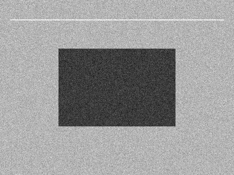
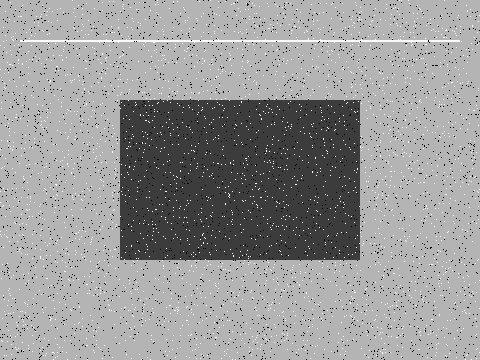
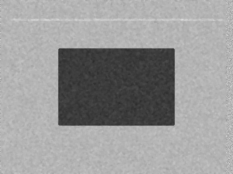
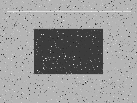
Throughout this chapter we use one synthetic test scene for all experiments: a dark rectangle on a uniform bright background (providing step edges), with a thin bright line only 2 pixels wide above it (simulating a fine structure such as a scratch or a bonding wire). Figure 6.1 shows the original scene and what it looks like under two typical kinds of noise.

6.1 Image Noise Models

To choose the right filter, you first have to understand what the noise looks like. The most common model in machine vision is additive Gaussian noise: the observed image \(g\) equals the true image \(f\) plus a random disturbance,

\[ g[n,m] = f[n,m] + \eta[n,m], \qquad \eta \sim \mathcal{N}(0, \sigma^2). \]

Every pixel is corrupted, but usually not by much — most of the disturbance falls within \(\pm 2\sigma\). Its physical origins are the sensor’s dark-current noise, readout noise, and the electronic noise introduced by amplifier gain. These factors are the superposition of many small independent disturbances, and by the central limit theorem their sum tends toward a Gaussian distribution. Figure 6.1 (b) shows exactly this situation — the image is “fuzzy” everywhere, but no single pixel is destroyed outright.

The other common kind is salt-and-pepper noise, also called impulse noise: a small fraction of pixels are randomly replaced by the minimum value (“pepper”, 0) or the maximum value (“salt”, 255), while the remaining pixels are entirely unaffected. Its sources include dead sensor pixels, transmission errors between the camera and the industrial PC, and isolated overexposed spots caused by specular reflection on highly reflective surfaces. The scattered black and white dots in Figure 6.1 (c) are typical salt-and-pepper noise — note that a corrupted pixel bears no relation whatsoever to its true value; the error can span the entire gray-level range.

Why do the two kinds of noise call for different filters? Gaussian noise means “everyone is slightly wrong” — averaging the neighborhood lets the errors cancel each other out. Salt-and-pepper noise means “a few are wildly wrong” — averaging only spreads the wild values to the neighbors. The right move is to discard the outliers, which is precisely what the median filter does.

The difference between these two models is far more than a mathematical curiosity: it directly determines the choice of filter. With Gaussian noise, every pixel’s observation is “roughly correct”; averaging the values in a neighborhood lets the independent zero-mean errors cancel, and the estimate improves — linear filtering is the natural choice. With salt-and-pepper noise, a corrupted pixel carries not “information with some error” but pure garbage; folding garbage into an average only contaminates the neighbors that were clean to begin with. What we need is a nonlinear mechanism that can recognize and discard outliers. The experiments later in this chapter will confirm this point again and again.

6.2 Linear Filtering and Convolution

The unifying mathematical form of linear spatial filtering is convolution. Given an input image \(f\) and a small template of weights — called the kernel \(h\) — the output image is

\[ g[n,m] = \sum_{k,l} f[n-k,\, m-l]\, h[k,l]. \]

Intuitively, the output value at \((n,m)\) is a weighted sum of a small input neighborhood centered at that point, with the weights given by the kernel. The kernel determines the filter’s entire character.

The simplest kernel is the mean filter kernel: a \(K\times K\) window in which every weight equals \(1/K^2\). For example, the \(3\times 3\) mean kernel is

\[ h = \frac{1}{9} \begin{bmatrix} 1 & 1 & 1\\ 1 & 1 & 1\\ 1 & 1 & 1 \end{bmatrix}. \]

Note the normalization factor in front of the coefficients: the sum of all kernel weights is called the filter’s DC gain. Normalizing the weights to sum to 1 means that filtering an image of constant gray value returns it unchanged — the average brightness of the image is preserved. This matters especially in measurement applications: if filtering quietly raised or lowered the overall gray level, every downstream algorithm that relies on gray-value thresholds or gray-value interpolation would be dragged along with it.

The mean kernel treats every pixel in the window equally, whereas the Gaussian filter assigns weights that decay with distance — the farther a pixel is from the center, the less it influences the output:

\[ h[n,m] = \frac{1}{2\pi\sigma^2}\exp\!\Big(-\frac{n^2+m^2}{2\sigma^2}\Big). \]

The parameter \(\sigma\) controls the spatial scale of smoothing: the larger \(\sigma\), the wider the effective neighborhood that participates in the average, the stronger the denoising — and the blurrier the image. Compared with the mean kernel, the Gaussian kernel has a monotonically decreasing frequency response with no sidelobe ringing, so its smoothing is “cleaner”; this makes it the default choice for linear denoising. In a discrete implementation, we sample the continuous Gaussian and then divide by the sum of the samples so that the DC gain is exactly 1.

In practice there are two further engineering points. First, the kernel size must match \(\sigma\). The Gaussian function extends infinitely in theory, but beyond \(3\sigma\) its amplitude is only about 1% of the central value, so it is usually truncated at \(K \approx 6\sigma\) (rounded to the nearest odd number): \(\sigma=1.2\) paired with a kernel of roughly \(7\times 7\) is sufficient. Too small a kernel clips the Gaussian’s shoulders; too large a kernel simply wastes computation. Second, the Gaussian kernel is separable: the two-dimensional Gaussian is exactly the product of a one-dimensional horizontal Gaussian and a one-dimensional vertical Gaussian, so one 2D convolution can be split into a horizontal 1D pass followed by a vertical 1D pass with identical results.

The payoff of separability: a \(K\times K\) 2D kernel costs \(O(K^2)\) multiply-adds per pixel, but split into two 1D kernels it costs only \(O(2K)\). At \(K=7\) that is 49 versus 14; at \(K=15\) it is 225 versus 30 — the larger the kernel, the bigger the savings. Virtually every commercial vision library implements Gaussian filtering this way internally.

6.3 Nonlinear Filtering

Linear filtering has one limitation it cannot escape: it cannot tell “noise” from “edges” — both are high-frequency content, so suppressing the former inevitably blunts the latter. Nonlinear filters step outside the weighted-average framework and thereby gain abilities that no linear method can have.

The median filter is the most important member of this family. Instead of computing a weighted sum, it sorts the pixel values in the window and outputs the median:

For each pixel (n, m) of the output image:
    take all pixel values in the K×K neighborhood centered at (n, m)
    sort these values in ascending order
    output ← the value in the exact middle of the sorted list (the median)

The median is naturally immune to outliers: if a few bad pixels of 0 or 255 land in the window, as long as they make up less than half of it, sorting pushes them to the ends of the list and they never get a chance to be the output. This is exactly the nemesis of salt-and-pepper noise. Moreover, when the median filter steps across a step edge, the majority of pixels in the window come from one side of the edge, and the output simply takes a representative value from that side — the edge stays sharp, with none of the transition band that linear filtering would smear out. The price it pays we will reveal in the experiments section.

The bilateral filter (Tomasi and Manduchi 1998) brings the edge-preserving idea into the weighted-average framework. The weight it assigns to each neighbor \(\mathbf q\) is the product of two Gaussian factors:

\[ g[\mathbf p] = \frac{1}{W_{\mathbf p}} \sum_{\mathbf q \in S} G_{\sigma_s}\!\big(\|\mathbf p-\mathbf q\|\big)\; G_{\sigma_r}\!\big(|f[\mathbf p]-f[\mathbf q]|\big)\; f[\mathbf q], \]

where \(W_{\mathbf p}\) is the sum of the weights (ensuring a DC gain of 1), \(G_{\sigma_s}\) is a Gaussian over the spatial domain, and \(G_{\sigma_r}\) is a Gaussian over the gray-value (range) domain. The intuition is crystal clear: for a neighbor to have a say in the output, it must satisfy two conditions at once — it must be nearby (high weight from the spatial Gaussian) and look alike (gray value close to the center pixel, high weight from the range Gaussian). In flat regions, neighbors have similar gray values and the bilateral filter degenerates into ordinary Gaussian smoothing, suppressing noise effectively. Near an edge, pixels on the opposite side differ greatly in gray value, the range Gaussian drives their weights toward zero, and averaging takes place only on the same side of the edge — so the edge is left untouched. \(\sigma_r\) draws the boundary of “one of us”: neighbors whose gray-value difference is below roughly \(2\sigma_r\!\sim\!3\sigma_r\) join the average, while those beyond it are treated as “the other side” and excluded.

6.4 Experimental Comparison

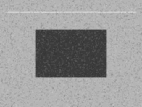
Now let the four filters compete head to head. First, their performance under Gaussian noise (Figure 6.1 (b)); the four filtered results are shown in Figure 6.2.

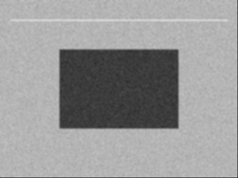
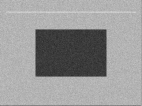
The mean and Gaussian filters both visibly flatten the grain, confirming the principle that “averaging cancels independent errors.” The price is equally visible: the rectangle’s edges are smeared into a gray transition band, and the 2 px thin bright line becomes dimmer and thicker, because its brightness has been spread across the surrounding background pixels. Comparing the two, at the same kernel size the Gaussian filter degrades the edges slightly less — a consequence of its weights being concentrated toward the center. The median filter keeps the rectangle’s edges remarkably sharp, but look at the thin bright line: it has all but vanished — a phenomenon we will discuss separately in a moment. The most balanced performer is the bilateral filter: the background noise is smoothed away, the rectangle’s edges stay crisp, and the thin line survives intact, because the gray-value difference between the line and the background (about 70 gray levels) far exceeds the \(\sigma_r=30\) “one of us” threshold — line pixels average only with line pixels. For Gaussian noise, the bilateral filter is the best choice for edge-preserving denoising.

Switch to salt-and-pepper noise (Figure 6.1 (c)), and the conclusions all but reverse; see Figure 6.3.

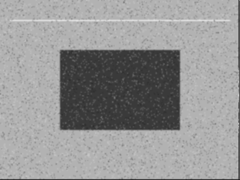
The mean and Gaussian results are disappointing: the impulses do not disappear — they get smeared. Each bad pixel of 0 or 255 shares its extreme value across the entire window, turning into a soft light or dark blotch about 5 px across, and the whole image ends up looking grimy. The median filter, by contrast, is overwhelmingly superior: the black and white bad pixels are removed wholesale, the background returns to uniformity, the rectangle’s edges remain sharp, and the result is nearly as clean as the original. This is the visual confirmation of the claim at the end of Section 6.1 — for outliers, discard, don’t average.

The result most worth remembering is the bilateral filter’s: it is nearly useless against salt-and-pepper noise. Compare Figure 6.3 (d) with Figure 6.1 (c): the bad pixels remain almost exactly where they were. The reason is no mystery, though it is often misunderstood: a salt pixel of value 255 differs from its surrounding background of about gray level 180 by 75 gray levels, far beyond the \(\sigma_r=30\) similarity threshold. In the bilateral filter’s eyes, this bad pixel is a “distinctive small structure” — none of its neighbors count as “one of us,” so it averages only with itself and naturally keeps its value. The bilateral filter’s edge-preserving mechanism becomes precisely a shield for impulse noise. When you face salt-and-pepper noise, reach straight for the median filter.

The median filter has its own bill to pay, however. Look again at Figure 6.3 (c) and Figure 6.2 (c) against the original in Figure 6.1 (a): the 2 px thin bright line has vanished in both median results. The reason is exactly the same one that removes the bad pixels — within a 5×5 window, the thin line contributes at most \(2\times 5=10\) pixels, fewer than half of the 25, so after sorting it can never occupy the median position, and it gets removed as “somewhat larger noise.” The median filter preserves edges, but not fine structures: any line-like or dot-like structure narrower than half the window width is wiped out, whether it is noise or a genuine target. This yields a hard constraint: the median kernel must be smaller than (twice) the width of the smallest structure to be preserved — if the thin line is 2 px wide, a 3×3 median kernel can still spare its life, but 5×5 will carry it away together with the noise. The filter does not know defects from noise; it only knows size.

6.5 SciVision Implementation

The four filters of this chapter are provided in the SciVision SDK by the SCIMV::SciSvFilter class, invoked as follows:

SCIMV::SciSvFilter f;
SciImage dst;
f.Mean(src, roi, &dst, 5, 5);
f.Gaussian(src, roi, &dst, 5, 5, 1.2, 1.2);
f.Median(src, roi, &dst, 5, 5);
// Bilateral(kernel diameter 9, spatial σ=3.0, range σ=30.0): neighbors whose gray-value difference exceeds ≈3σ get near-zero weight, hence edge-preserving
f.Bilateral(src, roi, &dst, 9, 3.0, 30.0);

Among the common parameters of these interfaces, src is the input image, roi restricts the processing region (production-line programs usually filter only the inspection region to save time), and dst receives the output. The filter-specific parameters are as follows.

kernelSizeX and kernelSizeY of Mean / Median (both 5 in the example above) are the window’s width and height; they must be odd so that the window has a center. The two may differ — for example, a flat (9, 3) window provides directional suppression of horizontal stripe noise.
Gaussian additionally accepts sigmaX and sigmaY (both 1.2 above), the horizontal and vertical Gaussian standard deviations. Remember the matching rule of Section 6.2: the window side should be roughly \(6\sigma\); pairing \(\sigma=1.2\) with 5×5 as above is a slightly tight truncation, acceptable in practice.
The three parameters of Bilateral are, in order, kernelSize (the neighborhood diameter, 9 above), space_sigma (the spatial-domain \(\sigma_s\), controlling the scale of “nearby”; 3.0 above together with diameter 9 satisfies the common ratio \(d\approx 3\sigma_s\)), and color_sigma (the range-domain \(\sigma_r\), controlling the “looks alike” threshold; 30.0 above means neighbors differing by more than about 90 gray levels get near-zero weight, so step edges above 70 levels are preserved almost intact).

The complete runnable project that generates all of this chapter’s experimental images is located at code/spatial_filtering/; readers can modify the noise levels and filter parameters to reproduce the results themselves.

Industry Case: Preprocessing for Scratch Detection on Metal Parts

In an inspection project for stamped metal parts, the sandblasted workpiece surface produced a large number of isolated bright specular spots whose statistics closely resembled salt-and-pepper noise. Initially a Gaussian filter was used for preprocessing: the specular spots were smeared into soft light-gray blotches that were hard to distinguish from scratches, and the false-detection rate was high. Switching to a 3×3 median filter removed the specular spots cleanly while keeping scratch edges sharp, and false detections dropped dramatically. A later “optimization” enlarged the median kernel to 7×7 — and the line immediately began missing fine scratches: the scratches were only 2–3 px wide, less than half the window’s population, and were removed as noise. This was the thin-bright-line experiment of this chapter replayed on the factory floor. Rule of thumb: choose the kernel at 2–3 times the noise-grain diameter, and keep it smaller than twice the width of the smallest defect; when the two conflict, preserving the defect comes first, and the residual noise is left to downstream area-based screening.

6.6 Summary

The key points of this chapter can be distilled as follows.

Identify the noise first, then choose the filter. Gaussian noise is “everyone slightly wrong,” suited to averaging-type linear filters; salt-and-pepper noise is “a few wildly wrong,” requiring discard-type methods such as the median filter.
The kernel of a linear filter should be normalized to a DC gain of 1, preserving the image’s average brightness. Truncate the Gaussian kernel at \(K\approx 6\sigma\), and exploit separability to cut the computation from \(O(K^2)\) to \(O(2K)\).
Bilateral filtering = spatial proximity × gray-value similarity, weighted together. It is the best edge-preserving denoiser under Gaussian noise; but isolated impulses are protected as if they were “edges,” so it is nearly useless against salt-and-pepper noise.
The median filter preserves edges but not fine structures: thin lines and small dots occupying less than half the window are wiped out together with the noise, so the kernel size must stay below twice the width of the smallest structure to be preserved.
Filter parameters are part of the measurement accuracy: kernel size and \(\sigma\) should be chosen from the noise scale and the smallest target size — not on the principle that “bigger is cleaner.”

For the systematic theory of spatial filtering (linear filters, order-statistic filters, and the link to the frequency domain), see the classic textbook by Gonzalez and Woods (Gonzalez and Woods 2018). The original construction of the bilateral filter is the paper by Tomasi and Manduchi (Tomasi and Manduchi 1998), cited several times in the body of this chapter, and the canonical edge-preserving advanced method of anisotropic diffusion originates with Perona and Malik (Perona and Malik 1990). For a more systematic treatment of smoothing filters in industrial inspection pipelines, see the book by Steger et al. (Steger, Ulrich, and Wiedemann 2018).