1 Digital Image Fundamentals

At the instant the lens focuses light onto the sensor’s active surface, the “image” is still a continuous physical quantity: every point on the image plane has its own illuminance, and brightness can take any real value. Yet what the image-processing program on the industrial PC receives is a matrix of integers. Between the former and the latter, two discretizations take place inside the camera: sampling — the sensor’s photosite array chops the continuous image plane into a finite grid of points, determining how finely the image resolves space; and quantization — the analog-to-digital converter compresses the continuous charge on each photosite into an integer with a finite number of levels, determining how finely the image resolves gray values. Each step throws away part of the information. The question this chapter answers is precisely this: when does the lost information not matter, and when does it come back to wreck an entire vision solution?

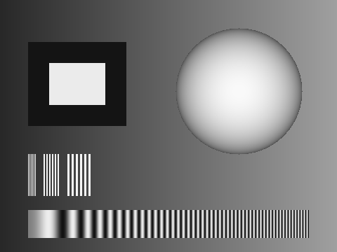
So that the consequences of both discretizations can be seen with the naked eye, this chapter constructs a 480×360, 8-bit grayscale test scene (Figure 1.1). A horizontal linear gradient background running from 40 to 160 and a Lambertian sphere provide smooth, continuous gray values — these are the most sensitive to quantization. A set of nested step rectangles (a dark 20 enclosing a bright 235) provides sharp edges. Groups of vertical bars 1, 2, and 3 pixels wide, together with a chirp stripe band whose frequency rises continuously from left to right, provide fine structures — these are the most sensitive to sampling. Every experimental figure that follows is genuinely generated by the programs under code/digital_images/.

Figure 1.1: The baseline test scene (480×360, 8-bit). Top left: a bright rectangle nested inside a dark one (step edges); top right: a Lambertian sphere (a continuous gray-value surface); the background is a horizontal gradient from 40 to 160; bottom left: groups of vertical bars 1/2/3 px wide; bottom: a chirp stripe band whose frequency increases to the right.

1.1 The Image as a Two-Dimensional Signal

Write the continuous image projected by the lens onto the sensor as \(f_c(x, y)\). Sampling turns it into a discrete image defined only on an integer grid,

\[ f[n, m] = f_c(m \Delta_x,\ n \Delta_y), \]

where \(n\) is the row index (increasing downward), \(m\) is the column index (increasing to the right), and \(\Delta_x, \Delta_y\) are the sampling intervals — physically, the pitch of the photosites. Quantization then restricts each value \(f[n,m]\) to a finite set of integer levels. A digital image is thus, in the end, a matrix of integers; the test scene of this chapter is exactly 360 rows × 480 columns.

This brings out the three most fundamental specifications. Resolution is the size of the sampling grid — the image’s width and height in pixels — and it sets the upper limit on spatial detail. Bit depth is the number of binary bits used to represent each pixel, which determines the number of gray levels — 8 bits give \(2^8 = 256\) levels, the most common output format for industrial cameras. Dynamic range is the ratio between the brightest and darkest signals the sensor can record simultaneously; bit depth determines into how many levels that range is divided for representation. The three are mutually independent: high resolution does not imply high bit depth, and a high bit depth does not mean the sensor can actually distinguish that many effective gray levels.

Common bit depths for industrial cameras are 8/10/12 bits. For most locating and inspection tasks, 8 bits is enough; but when an algorithm uses gray values as a physical quantity — for example, photometric stereo (Chapter 34) recovering surface normals from shading, or measuring the brightness uniformity of a backlight — the 256 levels of 8 bits are often insufficient, and 10-bit or even 12-bit output is required.

1.2 Quantization

Requantizing 256 gray levels down to \(L\) levels follows a simple rule: cut the gray axis into \(L\) segments of step size \(\Delta = 256 / L\), and record a pixel as level \(q\) if its value falls in the \(q\)-th segment:

\[ q[n, m] = \left\lfloor \frac{f[n, m]}{\Delta} \right\rfloor, \qquad \Delta = \frac{256}{L}. \]

The error introduced by quantization is at most half a step, \(\pm\Delta/2\), and is approximately uniformly distributed within each step — you can regard it as a kind of uniform noise superimposed on the image. It belongs to the same family of “perturbed gray values” as the sensor noise discussed in Chapter 6, except that it is determined by our own digitization and cannot be removed by averaging. The smaller \(L\), the larger the step, and the stronger this “noise”. Figure 1.2 shows the same scene quantized to 16 levels (4-bit, step 16), 4 levels (2-bit, step 64), and 2 levels (1-bit, step 128).

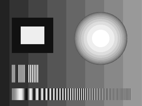
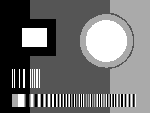
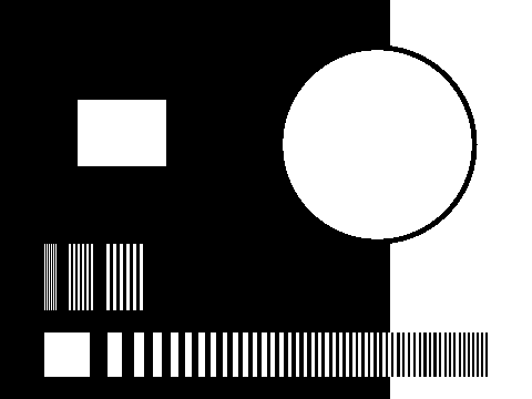
The first place quantization shows itself is not the edges but the smooth gradient regions. In Figure 1.2 (a), the gradient background breaks into clearly visible vertical banding artifacts, and the sphere turns into a set of concentric rings. The reason is not hard to see: the background climbs from 40 to 160 across 480 columns, so the gray-value difference between adjacent pixels is far smaller than the quantization step of 16. The continuous ramp is therefore sliced into a staircase of constant-gray plateaus, with a jump of a full step at each plateau boundary — and the human eye is extremely sensitive to large-area gray steps, so the banding is unmistakable. The sphere is the two-dimensional version of the same phenomenon: its constant-gray plateaus are ring-shaped, hence the concentric rings. Pressing on to 4 levels (Figure 1.2 (b)), the entire image is reduced to four shades of gray — classic posterization. At 2 levels (Figure 1.2 (c)) only a single threshold survives: most of the sphere and the brighter background on the right are both assigned to “white” and fuse into one region, and the sphere’s shape as an object is essentially lost.

Now look at the rectangles and the bar groups: down to 4-level quantization they remain crisply outlined. The gray-value difference across the step edge (20 versus 235) is far larger than the step size, so no matter where quantization places its cuts it cannot erase that contrast; the same holds for the fine bright bars (245) against the background. Edges and fine structures are insensitive to quantization; smooth gradient regions are the most sensitive. This conclusion maps directly onto bit-depth selection in engineering: inspection-type tasks built around edge finding, locating, and presence/absence checks care about high-contrast structures, and 8 bits is almost always enough; only measurement-type and photometric tasks, which must read information out of gentle gray-value variations, truly justify paying for higher bit depth.

1.3 Sampling and a First Look at Aliasing

Quantization loses gray values; sampling loses spatial detail. The intuitive criterion is: to resolve a periodic structure, at least 2 sampling points must land in each period — one for the bright half and one for the dark half — or the structure can slip through the gaps in the grid. This is the intuitive version of the sampling theorem; the rigorous frequency-domain statement is deferred to Chapter 11. When a structure is finer than this limit, it does not simply vanish — it masquerades as a coarse structure that does not exist. This phenomenon is called aliasing.

The experiment undersamples the scene spatially: keep 1 pixel out of every 4 (or every 8), with no prefiltering of any kind, then enlarge back to the original size by pixel replication for comparison. The equivalent resolutions are 120×90 and 60×45. The results are shown in Figure 1.3.

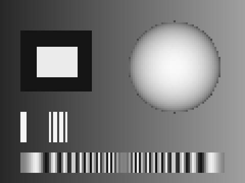
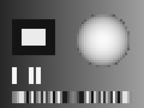
In Figure 1.3 (a), the two kinds of fine structure meet different fates, both equally bad. The 1 px bar group has a period of only 2 px, far below what a 4 px sampling interval can resolve: where a sampling point lands on a bar, the bar “exists”; where it lands in a gap, the bar vanishes. The result is that the original six neat thin bars either evaporate into thin air or fuse into one thick bar — a reader using this as a resolution target would reach a completely wrong conclusion. The chirp band is more deceptive still: its true frequency rises monotonically to the right, but in the undersampled image the stripes that should be densest on the right have instead become a set of slowly undulating coarse stripes. This “fake low frequency” is the standard face of aliasing — high-frequency structure beyond the sampling limit folds back and impersonates low frequency. The danger is that the result looks perfectly normal: the image is not blurred; it is simply wrong, and the original content cannot be recovered from the undersampled data after the fact. The 1/8 sampling of Figure 1.3 (b) pushes the destruction to the extreme: the bar groups are all but wiped out, the whole image turns into a strong mosaic of pixelation, and even the sphere’s outline becomes jagged.

The rule of thumb in industrial lens and camera selection that “pixel resolution should be at least half the minimum defect size” (i.e., the smallest defect spans ≥ 2 pixels) comes straight from the 2-samples-per-period criterion: only when a defect covers at least two pixels is it guaranteed to leave a detectable trace no matter where it falls on the grid. In practice the rule is often relaxed further to 3–5 pixels to leave signal-to-noise margin.

It is worth emphasizing that this experiment deliberately omits prefiltering. In a real camera, lens blur and the area integration of each photosite act as a natural low-pass prefilter that attenuates detail beyond the sampling limit before the photosites sample it, so aliasing is partly suppressed. Shrinking an existing digital image by “take every k-th pixel” decimation has no such protection — which is exactly why the engineering rule says “smooth before you downscale”. The systematic treatment is given in Chapter 11.

1.4 Color Images and Channels

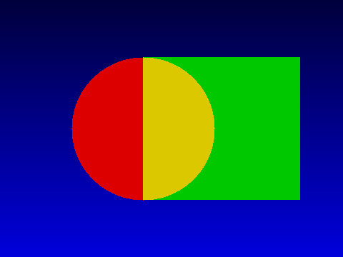
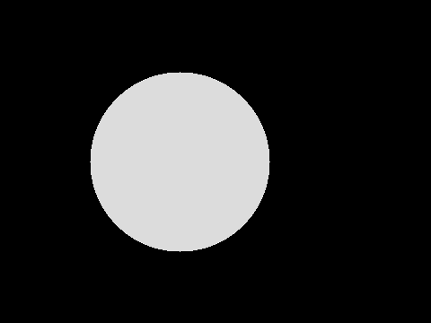
Structurally, a color image contains nothing new: an RGB image is simply three grayscale images of the same size — the red, green, and blue channels — stacked together. The synthetic scene of Figure 1.4 is drawn channel by channel: the blue channel is a vertical gradient background running 60→220 from top to bottom, the green channel is a rectangle of brightness 200, and the red channel is a disk of brightness 220. Where the disk and the rectangle overlap, red and green are both bright, and additive mixing renders the region yellow; extract the three channels individually and each one is an ordinary grayscale image.

There are two schemes for laying the three channels out in memory. Interleaved storage places the three components of each pixel contiguously, pixel after pixel, so one row occupies 3 times the width in bytes; planar storage keeps each channel as one contiguous grayscale block, with the three blocks placed one after another. The interleaved format makes it convenient to grab “the complete color of one pixel” and is the default for camera output and most image libraries; the planar format is convenient for whole-channel operations.

Interleaved storage carries one more detail you must watch: the order of the three components. In the SciVision SDK used throughout this book, the interleaved order of a 3-channel SciImage is BGR (byte 0 is blue) — the same convention as OpenCV’s default, and the reverse of the literal order “RGB”. This is stated nowhere in the SDK headers; we confirmed it empirically with a probe experiment. The first time this chapter’s color scene was generated, the disk came out blue and the background red — the classic symptom of a wrong channel-order assumption. Getting the channel order backwards raises no error, causes no crash, and the image even looks “normal” — red and blue are merely swapped — which is fatal to any sorting algorithm that relies on color.

The probe method: construct an image in which only a single channel is nonzero (e.g., write only byte 0), save it, and open it with a tool whose channel order is known (OpenCV or any image viewer); the displayed color tells you whether the undocumented SDK uses RGB or BGR. One experiment beats any amount of guessing.

Finally, the choice of whether to use color at all. The information color carries is intuitive to the human eye, but to an algorithm it means 3 times the data volume and bandwidth. Most industrial tasks — edge finding, locating, dimensional measurement, defect inspection — depend on brightness structure rather than hue, and a grayscale camera with well-designed lighting is usually the optimum. The cases where color is genuinely irreplaceable are tasks in which the targets differ only in color: identifying resistor color bands, sorting colored cables, checking color deviation in printed matter. Even with a color camera, the first step of many algorithms is to pick out the single channel with the best contrast and use it as a grayscale image.

1.5 Image Data Structures and SciVision

All images in this chapter’s experiments are constructed via SciImage on top of a memory buffer. The construction statements for the grayscale and color images are as follows (excerpted from code/digital_images/main.cpp):

SciImage img(copy.data(), W, H, W, 1, SCI_IMAGE_8U);        // grayscale: step = W
SciImage color(inter.data(), W * 3, H, W, 3, SCI_IMAGE_8U); // color: step = W*3

The full constructor signature is SciImage(unsigned char* data, int step, int rows, int cols, int channel, SciImageType depth). The six parameters, one by one:

data: the address of the pixel buffer. SciImage does not copy the data; the buffer’s lifetime must cover the entire period the image object is in use.
step: the number of bytes per row (the row stride). It is not “the number of pixels per row” — for a 1-channel 8-bit image it happens to equal the width W, but for a 3-channel image it is W * 3; and if each row of the buffer ends with alignment padding bytes, step must include the padding. When passing images between libraries goes wrong, nine times out of ten the bug is in step.
rows, cols: the number of rows (height H) and columns (width W). Note the constructor order: step first, then rows, then columns.
channel: the number of channels — 1 for grayscale, 3 for color; with 3 channels the data is interleaved in BGR order (the empirically verified finding of the previous section), and the writing code is:

for (int i = 0; i < W * H; ++i) {       // BGR interleaved (SDK order, verified by probe)
    inter[i * 3 + 0] = cb[i];
    inter[i * 3 + 1] = cg[i];
    inter[i * 3 + 2] = cr[i];
}

depth: the pixel-type enumeration (defined in SciDataDef.h). SCI_IMAGE_8U = 0 means 8-bit unsigned integers per channel — the 8-bit images this chapter has been discussing throughout; higher-bit-depth data corresponds to other values of the same enumeration.

The other core structure paired with SciImage is SciROI — the region of interest (ROI). In production-line images, usually only a small patch actually needs processing; restricting the algorithm to an ROI both saves time and avoids irrelevant interference, and the algorithm interfaces in nearly every later chapter of this book take an ROI parameter. How to generate the ROI dynamically from the workpiece’s actual position (position correction) is covered in detail in Chapter 19.

The complete runnable project that generates every experimental image in this chapter is located at code/digital_images/; readers can modify the quantization levels and sampling intervals to reproduce the results themselves.

Industry Case: 8-bit or 12-bit?

A backlight-panel brightness-uniformity measurement project initially chose an 8-bit camera. In the panel’s dark corner regions, all the gray values were squeezed into a dozen or so gray levels; the jump between adjacent levels alone consumed several percent of the measurement range, the resolution of the brightness computation fell far short of the acceptance requirement, and repeated measurements would not converge. After switching to a 12-bit camera, the same dark regions had 16 times as many gray levels, the measurement resolution immediately met the specification, and the problem was solved. But the cost was just as real: 12-bit pixels take 1.5 times the storage and transmission bandwidth, the camera’s frame rate dropped accordingly, and the image buffers along the entire pipeline had to be re-budgeted. The post-mortem conclusion: blindly choosing high bit depth for inspection-type tasks is pure waste — bit depth should be chosen according to the task’s need for gray-value resolution, not on the principle of “the higher the better”.

1.6 Summary

A digital image = sampling + quantization: sampling determines spatial resolution, quantization determines the number of gray levels (bit depth); the two lose information independently, and neither loss is recoverable.
Quantization hurts smooth gradient regions first (banding, concentric rings) while leaving step edges and high-contrast fine structures almost untouched — 8 bits is usually enough for inspection-type tasks, and only measurement-type and photometric tasks that use gray values as physical quantities need 10/12 bits.
Fine structures need at least 2 sampling points per period; when a signal is undersampled, high frequencies beyond the limit do not disappear — they alias into convincing fake low-frequency structures that cannot be repaired afterwards. Smooth before downscaling, and when selecting hardware make sure the smallest defect covers at least 2 pixels.
A color image is three grayscale images; with interleaved storage, always verify the channel order: the 3-channel SciImage in SciVision was empirically found to be BGR, with no mention in the headers — when integrating any SDK, one probe experiment beats guessing.
SciImage’s step is bytes per row, not pixels per row; multiple channels and row alignment both pull it away from the width value, making it the most common failure point when passing images across libraries.

A systematic treatment of sampling, quantization, and color spaces is given in (Gonzalez and Woods 2018), whose coverage of colorimetry and the various color models is especially complete; a modern perspective on image formation and digitization can be found in (Szeliski 2022). The rigorous origin of the sampling theorem’s “at least 2 samples per period” is Shannon’s foundational paper (Shannon 1949). For a more engineering-oriented treatment of image acquisition, sensor characteristics, and the digitization chain of industrial cameras, see the book by Steger et al. (Steger, Ulrich, and Wiedemann 2018).