33 Laser Triangulation
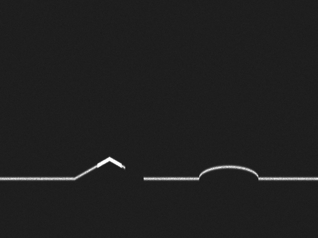
Structured light (Chapter 32) projects a whole sheet of coded texture onto an object and recovers the full-field height in a single exposure. Laser triangulation takes the opposite route: it casts out just one laser line, and a single exposure measures only the one profile where that line slices across the object. It seems like far less information, but paired with uniform motion of the object or the camera, stacking profile after profile along the scan direction reconstructs an entire 3D shape all the same — and the single-line scheme concentrates the light energy, keeps extraction simple, and runs blisteringly fast, making it the workhorse of online industrial 3D inspection: burr-height gauging on battery electrodes, weld reinforcement and undercut, profile wear on rails — behind most of these is a laser profilometer scanning the line at kilohertz profile rates. This chapter threads all of its experiments through one synthetic “profile target” scene (Figure 33.1): a flat conveyor belt carries a triangular prism and a circular-arc bump, a line laser strikes from above at a slant, and the camera looks down from another angle at the bright line that the objects lift up and bend.
33.1 The Triangulation Principle
What the laser emits is not a single beam but a sheet of light — a laser plane spread out by a cylindrical lens — which intersects the measured surface along a spatial curve. The camera observes this line from a direction making a fixed angle with the laser plane: when a surface point rises, the intersection shifts along the laser plane, which on the camera’s image plane appears as a row-direction displacement of the laser line in that column. Between height and displacement there is a one-to-one geometric relation — and this is exactly where the word “triangulation” comes from: the laser plane, the camera optical axis, and the measured point form a triangle, and given the baseline (the relative pose of camera and laser) and the observation angle, the depth of the third vertex can be solved.
After calibration, this geometry collapses into a single calibration constant. The synthetic data in this chapter takes the laser baseline row \(\text{BASEROW}=360\) (the laser row corresponding to the zero-height conveyor belt) and makes the row displacement proportional to the height, with proportionality coefficient \(k=0.8\ \text{px/mm}\). So when the laser line in some column lands on row \(r\), the height of that column is
\[ h = \frac{\text{BASEROW} - r}{k}. \]
A real system’s calibration curve need not be this linear, but the form is unchanged: extracting the row position of the laser line is equivalent to measuring the height. So the accuracy of laser triangulation, in the end, depends on a single thing — how precisely you can find the center of the laser line in each column.
The slanted laser plane is not parallel to the camera image plane, so with ordinary focusing only a short segment of the laser line is sharp and both ends are defocused. The Scheimpflug principle makes the lens plane, the image plane, and the laser plane meet along a common line, so the entire laser line falls within the depth of field at once — this is why profilometer lenses are commonly mounted tilted.
Compared with structured light, laser triangulation is a “single line vs. full field” trade-off: structured light measures the full field in one exposure, but must project multiple coded patterns, unwrap phase, and guard against crosstalk; laser triangulation measures only one line per frame and trades scanning for area, but pushes the signal-to-noise ratio and extraction accuracy of each line to the extreme. Both belong to active triangulation (Chapter 30); they simply place “information content” and “acquisition speed” on opposite pans of the scale.
33.2 Laser Line Extraction
Laser line extraction is a column-by-column, independent one-dimensional subpixel peak-localization problem: in each column’s gray profile, the laser line is a near-Gaussian bright peak, and what we want to estimate is the peak’s subpixel row coordinate. This is the same idea as the edge subpixel interpolation of Chapter 14 and the caliper localization of Chapter 20 — break an expensive two-dimensional localization into a string of cheap one-dimensional estimates, then cash in accuracy far beyond the pixel grid with subpixel interpolation. The two mainstream algorithms follow.
Center of gravity (CoG) treats the laser peak as a stretch of “mass distribution” and takes its gray-weighted centroid as the line center. Let the gray value of row \(r\) be \(I_r\) and the background estimate be \(b\); within a window near the peak,
\[ \hat r_{\text{CoG}} = \frac{\sum_r (I_r - b)\, r}{\sum_r (I_r - b)}. \]
It requires no model assumption and is extremely cheap to compute — the default implementation in industrial profilometers.
Gaussian fit assumes the laser cross section is a Gaussian peak \(I_r - b \approx a\,\exp[-(r-\mu)^2/2\sigma^2]\). Taking the logarithm of both sides yields a quadratic in \(r\), so one does a weighted parabolic fit of \(\ln(I_r-b)\) as \(\ln(I_r-b)=A+B(r-c_0)+C(r-c_0)^2\), and the peak position is given by the vertex
\[ \hat r_{\text{fit}} = c_0 - \frac{B}{2C}. \]
The fit adds a layer of model prior and is in theory more robust to noise, at the cost of more computation and a dependence on the assumption that “the peak really is Gaussian.”
The synthetic laser cross section in this chapter is Gaussian (\(\sigma=2\ \text{px}\), peak 220, background 30), with multiplicative speckle noise added — the random interference spots produced when coherent laser light hits a rough surface, whose intensity is proportional to the signal itself. This point is decisive for the contest between CoG and the fit below: multiplicative noise is strongest at the peak top, exactly the samples the fit weighs most.
Intuitively the Gaussian fit is “more sophisticated,” yet the measurements give a counterintuitive result. Comparing against ground truth column by column over the normal segment of Figure 33.1 (the unsaturated, unoccluded columns): CoG has a mean \(|\text{error}|=0.072\ \text{px}\), the Gaussian fit \(0.111\ \text{px}\) — the center of gravity actually wins by a hair. The reason lies precisely in speckle’s multiplicative character: the fit’s log transform amplifies the weight of weak-signal samples and also weighs the high-gray points near the peak top most heavily, and that is exactly where multiplicative speckle is fiercest; CoG takes a weighted average over the whole window and averages the random spots away, ending up more stable. This is an honest detail: there is no universally optimal extraction algorithm — it depends on the statistical structure of the noise. The next section shows that the fit’s real value only emerges when CoG fails outright.
33.3 Saturation: CoG’s Achilles Heel
Engineers often assume “the brighter the laser the better,” because brightness means a high signal-to-noise ratio. But gray values have a ceiling: an 8-bit sensor clips at 255. When the laser peak is clipped flat, disaster follows. Figure 33.2 compares two columns’ cross sections: the normal column is a complete, symmetric Gaussian peak, while the column at the prism apex, overexposed by specular reflection, has its peak top sheared off into a flat plateau — the symmetry information carried by the peak shape has been cut away.
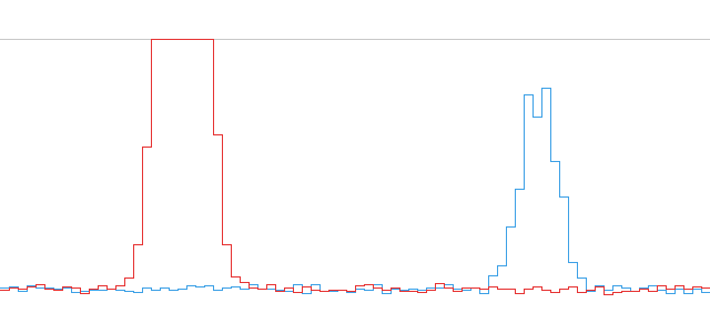
CoG is systematically biased on a clipped profile. It centers a window on the maximum pixel and takes the weighted average — but the plateau degenerates the “maximum pixel” into a whole stretch of tied highest points, and the centroid is dragged toward one side of the plateau, so the entire extracted line is pulled downward. The column-by-column statistics are striking: over the 49-column saturated segment, CoG has a mean \(|\text{error}|=0.387\ \text{px}\) and bias \(-0.387\ \text{px}\) — \(5.4\) times the normal segment, and entirely one-directional bias (not random jitter but a systematic low reading). Converted to height, the CoG estimate at the prism apex overestimates by \(+0.585\ \text{mm}\) relative to the truth. The Gaussian fit, by contrast, discards the clipped samples with \(I\ge250\) during fitting and uses only the unsaturated “Gaussian shoulders” on either side of the plateau to back out the peak position: the saturated segment’s mean \(|\text{error}|\) drops to \(0.078\ \text{px}\) with a bias of just \(+0.005\ \text{px}\), and the height error at the prism apex is \(-0.046\ \text{mm}\). Figure 33.3 draws this reversal clearly: inside the saturation band (yellow), CoG (red) collapses into the negative-error region, while the fit (blue) stays glued to the zero-error line throughout.
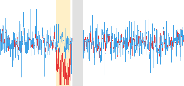
There is a reversal here that must be reported honestly. In the previous section’s normal segment, CoG (0.072) was still slightly better than the fit (0.111); the fit wins only when clipping destroys CoG. In other words, the fit is not “the more accurate algorithm” but “the algorithm more robust to saturation.” The lesson has two layers: first, the foremost red line of exposure is never to let the laser peak saturate — overexposure brings not a higher SNR but a systematic bias that cannot be repaired after the fact; second, when the profile may saturate, CoG silently overestimates the height, and for specular, glossy-painted, and other easily reflective surfaces one must switch to a fit that discards clipped samples, or flag the saturated columns separately.
33.4 Scanning and the Range Image
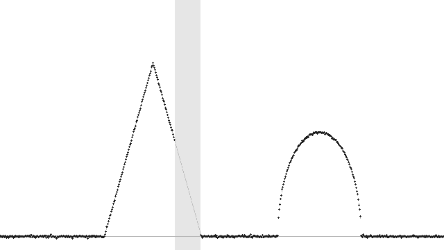
Feeding each column’s extracted laser-line row position into \(h=(\text{BASEROW}-r)/k\) turns one frame into a single height profile. Figure 33.4 overlays this reconstructed profile (black dots) on the ground truth (gray line): the triangular prism is a sharp-apex triangle and the circular-arc bump is a bow, both hugging the truth precisely; while over the segment shadowed by the ridge, the reconstructed profile is simply left blank — no laser means no data, and we never connect the gap with a fabricated curve.
A single profile is only one slice. Let the object pass uniformly through the laser plane on the conveyor belt and let the camera shoot continuously at a fixed frame rate, extracting one profile per frame and stacking them in order along the scan direction (rows), and you obtain a range image — where each pixel’s “gray value” is no longer brightness but the height at that location. It is a 2.5D representation between a two-dimensional image and a full three-dimensional point cloud: it has a regular pixel grid, but each cell carries a \(z\) value. Figure 33.5 is the range image stitched from this chapter’s 200 scan lines \(\times\) 640 columns, brighter for higher: the prism is a bright ridge with a slope, the circular-arc bump a soft bright spot.
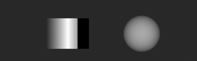
Note that pure-black vertical band to the right of the prism: the prism’s lower slope is blocked by its own ridge, the laser cannot reach it at all, and so the camera sees no bright line. In this frame 37 columns detect no laser peak, and the extraction algorithm faithfully flags all 37 columns as invalid (\(37/37\)), leaving an honest hole in the range image, never filled by interpolation. This is the exact opposite of the “silent failure” in Chapter 26: better to leave a visible hole than to fabricate a height whose falsity cannot be seen. Occlusion is a physical fact, and a fabricated smooth surface would lead downstream to misjudge a surface that simply does not exist. The whole range image has \(3700\) invalid pixels and a peak height of \(50.268\ \text{mm}\), all concentrated in the shadow region. The two profiles’ measurements also stand up to scrutiny: the prism measures \(49.954\ \text{mm}\) (truth 50) and the circular-arc bump \(29.918\ \text{mm}\) (truth 30), agreeing at the submillimeter level.
SciVision carries the range image with SciRangeImage: underneath are ushort raw counts, paired with three-axis resolutions resolutionX/Y/Z and an offset offsetZ; GetValue returns the raw count (not the \(z\)-scaled value), so the physical height must be obtained by multiplying by resolutionZ and adding offsetZ yourself; Save outputs a 16-bit PNG to preserve height precision. In this example GetValue reads \(49.940\ \text{mm}\) at the prism apex. It belongs, alongside SciPointCloud and SciTriangleMesh, to the core 3D data types of Sci3DData.
The range image is the bridge to point cloud processing in Part IX of this book: give each valid pixel its physical \((x,y)\) coordinate and \(z\) height, and the range image unfolds directly into an organized point cloud, with subsequent registration, segmentation, and measurement developed in Chapter 37.
33.5 Repeatability and Exposure
How good a height-gauging system is depends not only on how accurate a single measurement is, but more on the scatter of repeated measurements of the same spot — exactly the repeatability methodology emphasized in Chapter 20. We take 100 columns in a purely flat region, fix the geometry and vary only the random noise seed, repeatedly render and extract 50 times, compute the standard deviation of each column’s extracted position, and then average over all columns.
Laser brightness (exposure) is a double-edged sword here. At peak 220 (normal exposure), CoG’s standard deviation is \(0.091\ \text{px}\) (equivalent to \(0.114\ \text{mm}\)) and the fit’s \(0.139\ \text{px}\); dimming the laser to peak 100 raises CoG to \(0.112\ \text{px}\) (\(0.140\ \text{mm}\)) and the fit to \(0.163\ \text{px}\). The pattern is clear: the dimmer the laser, the lower the SNR, the worse the repeatability — underexposure is the source of random error. But the previous section told us that overexposure (saturation) brings a far more frightening systematic bias. Squeezed from both ends, exposure can only take a compromise: bright enough for sufficient SNR, yet not letting any column saturate. In practice one often tunes to “the highest real surface just barely not clipping” and keeps a saturation flag on anomalously reflective columns as a backstop.
33.6 SciVision Implementation
An SDK defect must be recorded faithfully. This book’s 3D laser-triangulation module SciSv3DLaserTriangle (v26.1) crashes with an access violation (0xC0000005) at every entry point on this machine: FindLaserLine (both overloads, every parameter combination), AnalysisLaserline, and ReconstructeImage — 20/20 crashes, regardless of whether fed a clean noise-free image, 8U or 16U, or any ROI (including the default UNDEF). So as not to let one crash drag down the whole example, the project isolates the SDK calls into a subprocess probe — the main process calls system("demo.exe sdkprobe") to spawn a child that pokes at the SDK, and a crash only makes the child exit abnormally, captured and logged by the main process; once some SDK version fixes it, the comparison result will automatically reappear. Laser line extraction is then done entirely with hand-written CoG and Gaussian fit (the source of all the numbers above).
// Subprocess probe: try the SDK entry (20/20 crashes here, kept as a baseline once the SDK is fixed)
SCIMV::SciSv3DLaserTriangle lt;
SciPointArray pts;  SciVarArray grays;
long rc = lt.FindLaserLine(img, roi, /*thresh*/60, /*width*/20, /*sigma*/3, &pts, &grays);
// rc!=0 records a failure; a child crash is caught by the return code of the main process's system()
On the range-image side, the construction and saving of SciRangeImage work fine and can be used with confidence:
// u16: raw count of each pixel's height (mm×100); resolution/offset are passed at construction
SciRangeImage ri(u16.data(), W, NSCAN, W * (int)sizeof(unsigned short), SCI_DATA_USHORT,
                 1.0, 5002.0, /*resZ*/0.01, /*offZ*/-0.01, /*resX*/XRES, 0.0, /*resY*/YSTEP, 0.0);
double v = ri.GetValue(100, 220);                 // raw count, not physical height
double z = v * ri.ResolutionZ() + ri.OffsetZ();   // → physical height mm
ri.Save("out\\range_image_sci.png");              // 16-bit PNG, preserves height precision
The expected interface of FindLaserLine is listed here as well, for reference once the SDK is fixed: input the laser image and the search ROI, give a peak-strength threshold, a laser line width, and a smoothing \(\sigma\), and output a string of subpixel laser points pts with corresponding gray values grays; the hand-written extraction in this example implements exactly the column-by-column CoG/Gaussian fit according to this semantics. The complete project that generates all of this chapter’s images and numbers lives in code/laser_triangulation/.
Industry Case: Burr-Height Inspection on Battery Electrodes
After lithium-battery electrode sheets are slit, burrs tens of microns high often remain along the edge; too tall a burr can pierce the separator and cause an internal short, so the burr height must be measured online and the part rejected. A line-laser profilometer scans across the electrode edge at kilohertz profile rates and should be more than capable of µm-level height gauging — but the electrode surface is mirror-like metal foil and coating, the laser striking it reflects strongly, and the peak easily shoots into saturation. Once clipped, CoG systematically overestimates the height by the mechanism revealed in this chapter: an edge that is not actually out of spec gets measured as a spuriously tall “burr,” causing mass false rejection (overkill). There are three countermeasures: first, suppress the reflection in hardware — lower the laser power and add a polarizer to suppress the specular component, bringing the laser peak back into the unsaturated range; second, switch the extraction algorithm from CoG to a Gaussian fit that discards clipped samples; third, flag the still-saturated columns separately and hand them to re-inspection rather than scrapping outright. The lesson is hard: for µm-level laser height gauging, the extraction algorithm matters as much as exposure control and the lens — even the most expensive profilometer, paired with an extraction algorithm that saturation biases, measures a false height.
33.7 Summary
- Laser triangulation trades a single line for extreme single-profile accuracy and stitches a full surface by scanning: the triangular geometry of the laser plane and the camera encodes height as the row displacement of the laser line (\(h=(\text{BASEROW}-r)/k\)); against structured light it is a “single line vs. full field, speed vs. information content” trade-off.
- Extraction accuracy decides everything, but no algorithm is universal: in the normal segment under multiplicative speckle, the center of gravity (CoG, 0.072 px) actually edges out the Gaussian fit (0.111 px) — the optimal extraction depends on the statistical structure of the noise and must be measured, not assumed.
- Saturation is CoG’s Achilles heel: a clipped profile biases CoG systematically (saturated segment \(-0.387\) px, height overestimated by \(+0.585\) mm, 5.4 times the normal segment), while the Gaussian fit drops to 0.078 px after discarding clipped samples. The foremost red line of exposure is never to let the laser peak saturate.
- Occlusion should leave an honest hole, never interpolate: in the range image all 37 occluded columns are flagged invalid — better empty than fabricated, since a faked smooth surface is far more dangerous than a visible hole.
- Exposure is a compromise between underexposure’s random error and overexposure’s systematic bias: at peak 220 CoG’s repeatability is 0.091 px, rising to 0.112 px when dimmed to 100; the tuning target is “the highest real surface just barely not clipping.”
The theoretical foundation of subpixel laser-line extraction is the unbiased curvilinear-structure detector proposed by Steger (Steger 1998), which yields subpixel centerline localization together with width estimation; a fast and robust laser-stripe extraction method for the reflections and noise of industrial sites is given by Usamentiaga et al. (Usamentiaga, Molleda, and García 2012). A more systematic treatment of laser triangulation and 3D reconstruction can be further consulted in the book by Steger et al. (Steger, Ulrich, and Wiedemann 2018).