36 Confocal Imaging and Focus Variation
By the time Part VIII reaches this point, the previous five 3D-imaging techniques have each leaned on one geometric or optical constraint to convert height into a measurable image quantity: stereo relies on disparity, structured light and deflectometry rely on phase, laser triangulation on displacement, photometric stereo on shading. They share one thing in common — all of them treat the lens’s depth of field as an ever-welcome ally, the bigger the better, wishing the entire measurement range could be sharp everywhere. This chapter does the opposite, turning the “defect” of limited depth of field into the very means of measurement: the lens renders only the object plane that is exactly in focus sharp, so scan layer by layer along the optical axis, see at which layer each pixel is sharpest, and the Z position of that layer is the height of the point. In a sentence — “wherever it is sharpest, that is where the object sits in height.” This is focus variation (also called shape from focus), together with its cousin, confocal microscopy, which physically rejects out-of-focus light with a pinhole. They are slow and have a small field of view, yet they are the workhorses of microscale topography measurement: surface roughness, the cutting-edge radius of a tool, the step heights of microstructures — measuring these down to the submicron relies on this family of methods.
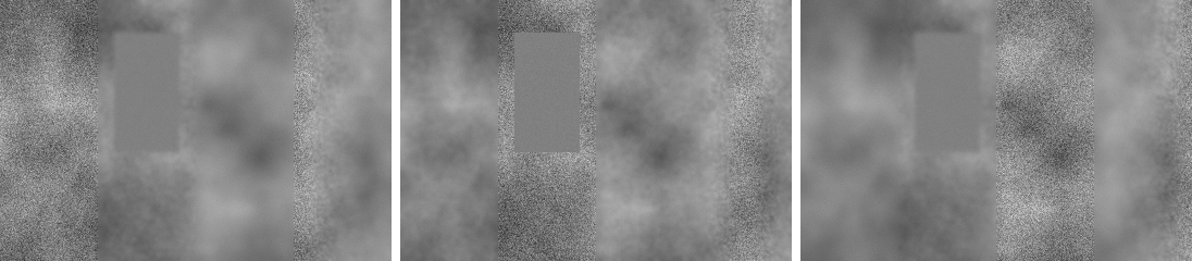
Figure 36.1 is this chapter’s starting point — slices of the same staircase surface captured at three focus heights. Note carefully: as the focus plane rises, the left, middle, and right step segments sharpen in turn, while the patch in the figure that stays smoothly blurred throughout is exactly the “failure region” that the second half of this chapter will discuss at length.
36.1 Principle of Focus Variation
Recall the discussion of depth of field and sharpness in Chapter 3: an object point converges to a sharp point on the image plane only when it lies within the depth-of-field range near the focus plane; the farther it deviates from the focus plane, the larger the circle of confusion, and the blurrier the image. To quantify this: if the object point’s height is \(h\) and the focus plane is at \(z\), then the larger the defocus \(|z-h|\), the more the high-frequency detail in the point’s neighborhood is wiped flat. This chapter’s synthetic data is modeled exactly on this physics — each slice applies to every pixel a space-varying Gaussian blur of standard deviation \(\sigma=0.4\,\text{px}\) per 10 μm of defocus, so that at focus \(\sigma\to 0\) and the texture is sharpest.
The measurement procedure then becomes clear: acquire a stack of images at fixed intervals along the optical axis, forming a focus stack; for each pixel, compute a focus measure value layer by layer, yielding a sharpness curve along \(z\); the \(z\) corresponding to the curve’s peak position is the height of that pixel.
The sharpness operator has to answer “how sharp is this neighborhood,” which in essence is measuring local high-frequency energy — sharing the same root as the gradient operators of Chapter 13. Two families are common in engineering: Tenengrad (the sum of squared Sobel gradient magnitudes) and the sum of modified Laplacian (SML). This chapter’s implementation adopts the latter: first, for each pixel, take the sum of the absolute values of the second differences in the x and y directions,
\[ \text{ML}(x,y) = \big|\,2I(x,y) - I(x{-}1,y) - I(x{+}1,y)\,\big| + \big|\,2I(x,y) - I(x,y{-}1) - I(x,y{+}1)\,\big|, \]
the reason for taking absolute values before summing (rather than summing directly as the ordinary Laplacian does) is to avoid the x- and y-direction curvatures cancelling each other when they have opposite signs; then sum ML within a \(9\times 9\) window around each pixel to obtain that pixel’s sharpness at that layer. The window sum is the crucial step — the single-pixel second difference is extremely sensitive to noise, so neighborhood aggregation is needed to “flatten and smooth” the sharpness curve, making the peak stable.
Why does focus variation measure only height relative to the stack, with no external calibration scale needed? Because it does not ask “how far is this point from the camera” but “at which layer is this point sharpest” — the layer index times the known slice spacing is the physical height. The Z-axis accuracy is therefore determined entirely by the stepping accuracy of the scanning stage, independent of the lens’s lateral calibration. This is also why it can easily reach submicron at the microscale: getting one mechanical step accurate is far easier than calibrating a whole imaging geometry accurately.
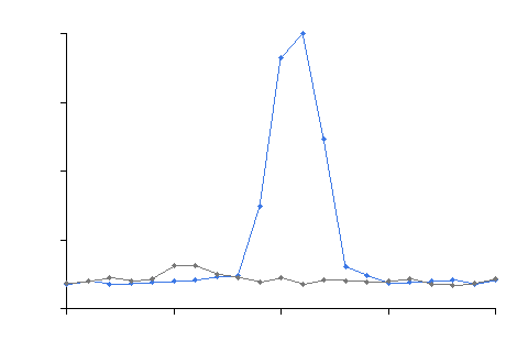
Figure 36.2 plots this sharpness curve. The blue one comes from a textured, sharp pixel (plateau C, true height 100 μm): the sharpness rises then falls with \(z\), forming a clear peak at \(z\approx 100\,\mu\text{m}\) — wherever the peak is, the height is. The gray one is left for Section 36.3.
36.2 Quantization and Subpixel
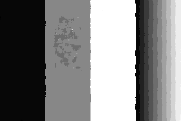
Taking “the layer with maximum sharpness” directly as the height immediately runs into an accuracy ceiling: the slice spacing itself is the quantization step. This chapter’s stack has 21 layers spaced 10 μm apart, so the coarse height can only be …, 90, 100, 110… these integer multiples of 10 (offset by a −7 μm stage-origin shift), and any detail with a height difference of less than 10 μm gets merged into the same layer. Figure 36.3 plots the coarse height map — a ramp that should be a continuous transition is sliced into 10-μm-wide contour terraces (terracing), looking just like a topographic contour map. This is exactly the shape of quantization error.
The way to break past quantization is the subpixel triad idea that recurs throughout this book (used by the edges of Chapter 14 and the calipers of Chapter 20): the true peak almost never lands exactly on a sample point, but its true position is hidden in the shape of the curve near the peak. Concretely, fit a parabola to the sharpness values \((f_{k_p-1}, f_{k_p}, f_{k_p+1})\) of the peak layer \(k_p\) and its two neighbors, and take the vertex as the sub-layer peak position:
\[ \delta = \frac{1}{2}\,\frac{f_{k_p-1} - f_{k_p+1}}{f_{k_p-1} - 2f_{k_p} + f_{k_p+1}}, \qquad h = (k_p + \delta)\cdot \Delta z + z_0, \]
where \(\delta\in[-1,1]\) is the sub-layer offset relative to the peak layer and \(\Delta z=10\,\mu\text{m}\) is the slice spacing. This step liberates the height from “integer multiples of 10 μm” to a continuous value. Figure 36.4 is the refined height map — the terraces are gone, the ramp is restored to a smooth transition, and the three plateaus become clean.
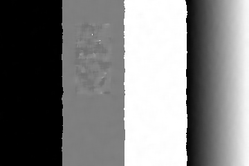
The numbers are honest. On the three flat plateaus, the height RMS error drops from the quantized 3.000 μm to the subpixel 0.342 μm, an improvement of 8.8×; the ramp region on the right drops from 2.933 μm to 0.442 μm, an improvement of 6.6×. The step heights (differences of the mean subpixel heights of the three plateaus) measure B−A = 49.935 μm, C−B = 50.044 μm, C−A = 99.980 μm, essentially exact against the true values 50 / 50 / 100 μm — submicron step measurement, “interpolated” out of a 10 μm quantization grid just like this.
The premise of parabolic interpolation is that the curve near the peak is approximately symmetric and twice differentiable. When the slice sampling is too sparse (the peak spans only two or three layers) or the curve is gnawed ragged by noise, this assumption loosens and the \(\delta\) estimate distorts accordingly. Engineering offers two countermeasures: take the slice spacing denser when scanning (let the peak span more than 5 layers), and smooth the sharpness curve lightly before interpolating. This chapter’s 1.5-graylevel readout noise is exactly there to make this subpixel gain withstand the test of noise — clean, noise-free synthetic data would overestimate the real accuracy.
36.3 Texture Dependence
Focus variation has one fatal premise, already spoiled by the gray curve of Figure 36.2: the sharpness curve must have texture before it can have a peak. The sharpness operator measures the decay of local high-frequency energy with defocus; but if a pixel’s neighborhood has no high-frequency content of its own — a uniform, polished, textureless surface — then whether in focus or not, its sharpness stays close to a low, flat constant. With no peak in the curve, the whole logical chain of “peak position = height” breaks: the algorithm can only pick some maximum at random from a field of noise as the peak, and the height it gives is purely random.
Figure 36.5 is the confidence mask: using a peak prominence (normalized peak height) of 0.5 as the threshold, it paints the untrustworthy pixels black. The result is intuitive — the texture-poor patch inside plateau B is masked out as a whole. The quantitative contrast is equally stark: the valid rate of the texture-poor region is only 18.7% (1232/6600), whereas the region with normal granite procedural texture reaches a valid rate of 100% (14700/14700). This failure region is not a contrived counterexample; it is simply a textureless patch on the same solid surface — in reality, polished surfaces, mirror surfaces, and large smooth painted surfaces are full of it everywhere.
“No texture → failure” is the same hurdle running through the 3D part of this book, only wearing three different faces: the stereo of Chapter 31 cannot find left-right correspondences in textureless regions and the depth map opens holes; Chapter 32 simply actively “prints” striped texture onto the surface to bypass it; this chapter’s focus variation gets no sharpness peak in textureless regions. The physical mechanisms of failure differ across the three (matching ambiguity / no passive texture / no high frequency to decay), but the root cause is the same: the surface has no local structure for the algorithm to “grab.” Remember this isomorphism, and on encountering a smooth surface you will reflexively ask first, “where does my texture come from?”
There are only two countermeasures, just as for stereo and structured light: either actively create texture — project structured illumination, spray a matting agent, “plant” high frequency onto the surface; or honestly admit failure — use a confidence threshold to reject the untrustworthy points, never letting a random peak position contaminate downstream measurement. Taking the garbage heights of a textureless region as real is far more dangerous than leaving a hole.
36.4 Optical Sectioning in Confocal
The previous sections were all about focus variation, relying on an algorithm to find the sharpness peak in the focus stack after the fact. True confocal instead solves the same problem at the optical physics level, and the two must be honestly distinguished — this chapter’s experiment does the former, while the latter described in this section has no accompanying simulation.
The core of confocal is a pair of conjugate pinholes. A point light source illuminates through a pinhole and is focused onto a point on the object plane; the light reflected or fluoresced from that point is then converged by the objective and can reach the detector only by passing through a detection pinhole that is optically conjugate to the illumination pinhole. The key is this: only light from the point on the focus plane converges exactly onto the detection pinhole and passes through smoothly; out-of-focus light from above or below the focus plane forms a diffuse spot at the pinhole plane, and the vast majority of it is blocked by the pinhole. Thus the signal the detector receives comes almost entirely from the thin, current layer in focus — this is optical sectioning. Scanning point by point (point-scanning confocal sweeps the whole field with a galvanometer or spinning disk) and then changing the focus-plane height layer by layer, one can “slice” out the 3D structure layer by layer.
Compared with focus variation, the difference is plain at a glance: confocal physically rejects out-of-focus light in the light path with a pinhole, so each layer’s signal itself contains only focus-plane information, and the axial resolution is set by the optical diffraction limit, reaching submicron or even better; focus variation relies on an algorithm to find the sharpness peak after the fact in the full image containing defocus, so out-of-focus light always participates in imaging, and the accuracy is constrained by the sharpness operator and the texture quality. Each has its niche: confocal is high in accuracy with clean sectioning, but point-scanning is slow and the equipment expensive, and it still requires the measured surface to return enough signal; focus variation works with just an ordinary microscope plus a Z-scanning stage, and since the area sensor images a whole layer at once it is far faster, at the price of a heavy dependence on surface texture. In a sentence — choose confocal when accuracy comes first, choose focus variation when speed comes first and the surface has texture.
36.5 SciVision Implementation
This is worth recording specially: after a string of SDKs in this book’s 3D part that “fell silent with no output / crashed” (phase measurement, laser triangulation, and photometric stereo, not one of which was usable), SCIMV::SciSv3DFocus is the rare usable case — it really did return a valid depth map. The procedure is two steps: CalGradArray first computes the focus stack layer by layer into a stack of gradient (sharpness) maps, and CalDepthMapByFocusStack then outputs a SciRangeImage depth map from it.
SCIMV::SciSv3DFocus fo;
SciImageArray grad;
fo.CalGradArray(arr, 21, &grad);              // per-layer sharpness (gradient) maps of the focus stack, meanSize=21
SciRangeImage depth; SciImage color;
fo.CalDepthMapByFocusStack(arr, grad, 31, 31, // smoothing window 31×31
                           1.0, 1.0, ZSTEP,   // x/y resolution, z slice spacing (μm)
                           0, false, 1,
                           &depth, &color);
double z = depth.GetValue(row, col) * depth.ResolutionZ() + depth.OffsetZ();
But it has one clear shortcoming: the depth is quantized to the nearest slice, with no subpixel. Verifying on the sample points shows that the heights the SDK gives land exactly on the slice integer multiples 10 / 60 / 110, with none of the sub-layer interpolation of Section 36.2. This constitutes an honest and rare favorable comparison: the hand-written parabolic interpolation (submicron) is strictly better than the SDK’s 10 μm quantized output — not because the SDK crashed, but because it only got as far as “take the nearest layer.” This chapter’s code therefore walks on two legs: use the SDK to verify that this stack-based height-measurement path works, then use a hand-written sharpness operator plus peak interpolation to push the accuracy to submicron. Below are the two core fragments of the hand-written part — sharpness (SML window sum) and the parabolic interpolation of the peak:
// modified Laplacian: take absolute values of the x/y second differences before summing (to avoid sign-cancellation)
float lx = std::fabs(2.0f*I[c] - I[c-1] - I[c+1]);
float ly = std::fabs(2.0f*I[c] - I[c-W] - I[c+W]);
ml[c] = lx + ly;                              // then sum within a 9×9 window to get the SML sharpness

// parabola vertex → sub-layer peak position δ ∈ [-1,1]
double den = a - 2*b + c;                     // a,b,c = sharpness of the layers left-of-peak / peak / right-of-peak
if (std::fabs(den) > 1e-9) delta = 0.5*(a - c)/den;
double h = (kp + delta)*ZSTEP + ZBASE;        // continuous height (μm)
Industry Case: Micro-Measurement of Cutting-Tool Edges
The edge quality of a carbide milling cutter directly determines its cutting life, requiring micron-level measurement of the edge-arc radius and chipping notches. A production line used focus variation under a microscope to quickly build a focus stack of the edge, producing a height map in a few seconds, a cycle time far better than point-by-point confocal scanning. The problem arose on the polished back of the edge: there the surface was smooth, the local texture insufficient, the sharpness curve flat, and the height map showed patches of random jumps, “measuring” gullies that simply do not exist into what should be a smooth edge face. The countermeasure had two layers: first, add a beam of structured illumination to the edge, projecting onto the smooth face high-frequency texture for the sharpness operator to grab; second, use a peak-prominence threshold to reject the points that are still untrustworthy, preferring to leave holes over outputting garbage. The lesson is direct — focus variation’s speed advantage is premised on texture; when you meet a textureless place, either create texture or switch to confocal.
36.6 Summary
This chapter turned “limited depth of field” from a defect into a means of height measurement, with the key points as follows.
- The peak is the height. Acquire a focus stack along the optical axis, compute a per-layer sharpness curve for each pixel, and the Z corresponding to the peak position is the height; the sharpness operator (Tenengrad / modified Laplacian) is in essence a measure of local high-frequency energy, sharing the same root as the edge gradient.
- The slice spacing is the quantization step. Taking the peak layer directly can only give staircase-like heights at integer multiples of 10 μm; a parabolic interpolation over the three layers near the peak yields the sub-layer peak position, and this chapter measured the flat-region RMS dropping from 3.000 μm to 0.342 μm (8.8×), with step measurements accurate to 49.935 / 50.044 / 99.980 μm.
- Focus variation depends heavily on texture. The sharpness curve of a textureless region is flat with no peak, and the peak position is decided by noise (texture-poor region valid rate 18.7% vs textured region 100%); it must be rejected with a confidence threshold, or remedied by actively projecting texture — this is the same hurdle as the textureless failure of stereo and structured light.
- Confocal and focus variation share a root but diverge in path. Confocal relies on conjugate pinholes to optically reject out-of-focus light and do hard sectioning, submicron in accuracy but slow; focus variation relies on an algorithm to find the sharpness peak after the fact, fast but texture-dependent. Choose the former when accuracy comes first, the latter when speed comes first and there is texture.
- A rare usable SDK case.
SciSv3DFocusreturns a valid depth map, but quantized to the nearest slice with no subpixel — hand-written peak interpolation is strictly better, constituting an honest favorable comparison.
The foundational work of focus methods is Shape from Focus proposed by Nayar and Nakagawa (Nayar and Nakagawa 1994); a systematic comparison and evaluation of the various sharpness (focus-measure) operators is given by Pertuz et al. (Pertuz, Puig, and Garcia 2013). A systematic treatment of focus variation and confocal (the comparison of sharpness operators, the details of confocal optics) can be further consulted in the book by Steger et al. (Steger, Ulrich, and Wiedemann 2018). With this, all six 3D-imaging techniques of Part VIII are complete: stereo and focus variation are passive / weakly active, while structured light, laser triangulation, photometric stereo, and deflectometry are active; laser triangulation and structured light target the macroscopic millimeter scale, while confocal specializes in the microscopic micron scale; the first five each serve diffuse surfaces, while deflectometry alone guards the specular. No single one of the six techniques does it all — each has its own failure boundary (no texture, specular interreflection, occlusion, non-Lambertian, transparent, speed), and the essence of 3D selection is to first recognize which boundary your workpiece falls outside of.