13 Edge Detection
The most information-dense places in an industrial image are where the gray value becomes discontinuous: the boundary between workpiece and background, the contour of a hole, the strokes of a character, the two sides of a scratch — nearly all the geometric information needed for locating and measurement is carried by these edges. The gray value of a flat region drifts with the illumination, but the position of an edge stays comparatively stable — which is why visual measurement places its trust in edges. Chapter 14 solved the one-dimensional problem of “we roughly know where the edge is; localize it precisely along a search line”; this chapter answers the more fundamental question — when we do not know in advance where the edges are, how do we find all of them in the entire image and obtain a two-dimensional edge map? The edge map is the standard input to downstream algorithms such as contour analysis, shape matching, and the Hough transform of Chapter 15.
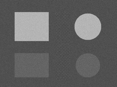
The experiments of this chapter run on a single 480×360 synthetic scene (Figure 13.1): on a background of gray value 80, the upper part holds a pair of high-contrast shapes — a rectangle and a circle at gray value 180 (contrast 100); the lower part holds a pair of low-contrast shapes at gray value 100 (contrast only 20); squeezed between the two columns of shapes is a vertical texture band, a two-dimensional sinusoidal texture of amplitude ±5 and period 12 px (simulating surface textures such as brushed metal or woven fabric); the whole image is overlaid with Gaussian noise of standard deviation \(\sigma=8\) (random seed fixed for reproducibility). Strong edges, weak edges, texture, and noise compete in the same arena — a good edge detector should report the first two and reject the last two.
13.1 The Gradient and First-Order Operators
An edge is a rapid change of gray value along some direction, and “rate of change” is precisely the derivative. For a two-dimensional image, combining the horizontal and vertical partial derivatives gives the gradient \(\nabla f = (g_x, g_y)\): its direction points where the gray value rises fastest, and its magnitude measures how violent the change is. A discrete image has no true derivatives; we can only approximate them by differences of neighboring pixels. The most widely used approximation is the Sobel operator — a pair of \(3\times 3\) convolution kernels:
\[ h_x = \begin{bmatrix} -1 & 0 & 1\\ -2 & 0 & 2\\ -1 & 0 & 1 \end{bmatrix}, \qquad h_y = \begin{bmatrix} -1 & -2 & -1\\ 0 & 0 & 0\\ 1 & 2 & 1 \end{bmatrix}. \]
\(h_x\) takes a central difference in the horizontal direction and a \([1\ 2\ 1]\)-weighted smoothing in the vertical direction; \(h_y\) does exactly the opposite. Differencing and smoothing run perpendicular to each other — differentiation itself amplifies noise, so averaging first in the direction perpendicular to the derivative is a way of using the tools of Chapter 6 to “insure” the difference.
The Sobel kernels are separable: \(h_x = [1\ 2\ 1]^{\mathsf T} \otimes [-1\ 0\ 1]\), i.e. “vertical smoothing × horizontal differencing.” Replace the smoothing part with \([1\ 1\ 1]\) and you get the Prewitt operator; replace it with \([3\ 10\ 3]\) and you get the Scharr operator with better rotational symmetry — the skeleton is always “smooth in one direction, difference in the other.”
The two components yield the gradient’s magnitude and direction:
\[ A = \sqrt{g_x^2 + g_y^2}, \qquad \theta = \operatorname{atan2}(g_y,\, g_x). \]
The magnitude answers “how edge-like is this,” the direction answers “which way does the edge run” (the gradient direction is perpendicular to the edge’s course), and the Canny pipeline will need both.
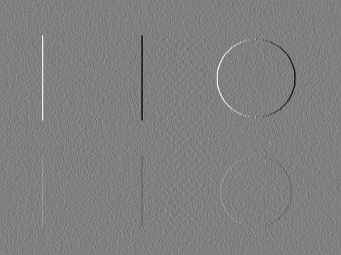
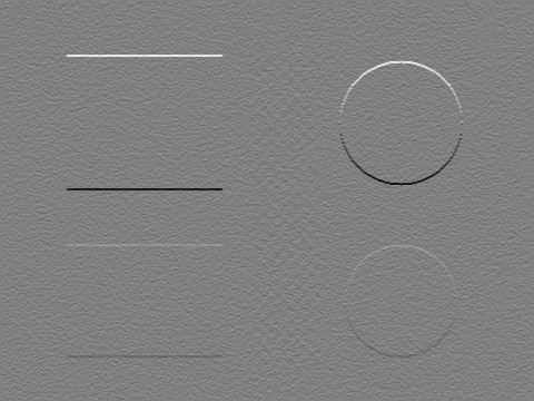
First, observe the directional selectivity of the components. Figure 13.2 shows the two signed components of a \(3\times 3\) Sobel applied to the test scene (displayed with an offset of 128 and a scale of 1/4: brighter than mid-gray is positive, darker is negative). \(g_x\) lights up only the vertical edges: the rectangle’s left edge is positive (crossing from 80 into 180, gray value rising) and its right edge negative; the circle’s ring is bright on the left and dark on the right — the same circle, opposite gradient directions on its two sides; the rectangle’s top and bottom edges vanish completely in \(g_x\). The behavior of \(g_y\) is exactly the transpose: it sees only horizontal edges, positive on top, negative on the bottom. The responses of the low-contrast shapes are only 1/5 of the strong ones and look dim in both images — the edge response is proportional to contrast, and this plain fact is the root of every thresholding problem to come.
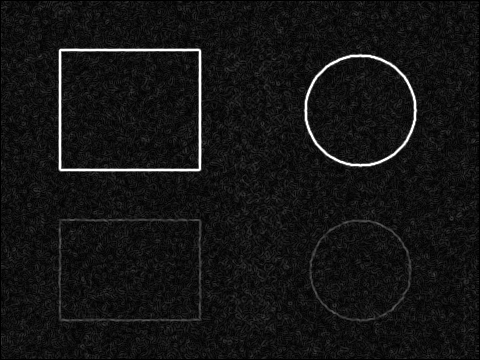
Combining the two components into the magnitude, the directional information disappears and all edges brighten alike, giving Figure 13.3 — this is the direct output of the SDK’s SobelAmplitude. The strong contours are crisp and bright, the weak contours faintly discernible, and the background is carpeted with the granular response of noise: differentiation amplified the noise, and with a first-order operator alone we obtain only a grayscale map of “edge likelihood” — still several crucial steps away from a clean edge map.
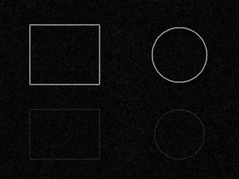
SobelAmplitude, SUM_SQRT combination). Strong contours bright, weak contours dim, and the background carpeted with the granular response caused by noise.
13.2 A Second-Order Operator: Laplace
The other line of attack is the second derivative. The Laplacian is the sum of the second derivatives in the two directions, \(\nabla^2 f = \partial^2 f/\partial x^2 + \partial^2 f/\partial y^2\), with the 8-neighborhood discrete kernel
\[ h = \begin{bmatrix} 1 & 1 & 1\\ 1 & -8 & 1\\ 1 & 1 & 1 \end{bmatrix}. \]
Its selling point is localization by zero crossing: across a step edge, the first derivative is a single peak, while the second derivative has one extremum on each side of the peak and passes through zero exactly at the edge position — detecting the zero crossings should, in theory, yield naturally closed, single-pixel-wide edge contours with no direction to choose.
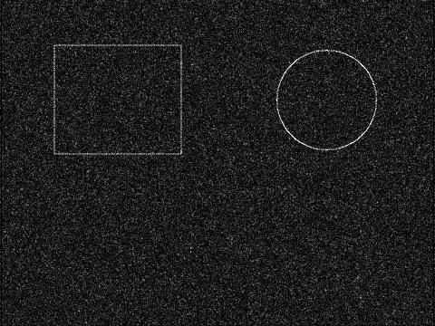
The measurements, however, pour cold water on this idea. Figure 13.4 shows the response of the SDK’s Laplace (\(3\times 3\), 8-neighborhood kernel, absolute-value output) on the test scene: the entire image is drowned in noise grain, and the strong contours survive only as faintly visible double lines — the second derivative has one extremum on each side of the edge, which under absolute-value display becomes two parallel streaks of response flanking the true zero-crossing position in between. The weak contours sink into the noise entirely. Two causes compound: first, second-order differencing amplifies high-frequency noise far more than first-order differencing does, and once the \(\sigma=8\) noise has been churned through it, the useful signal is gone; second, the Laplacian provides no directional information, so downstream processing cannot refine along the edge normal the way the gradient allows. This is why first-order operators dominate absolutely in industrial practice — the theoretical elegance of the second-order operator is no match for its fragility to noise.
The classic remedy that makes second-order operators practical is LoG (Laplacian of Gaussian): smooth with a Gaussian first, then take the Laplacian, which is equivalent to a single convolution with a “Mexican hat”-shaped kernel; its difference approximation, DoG (the difference of two Gaussians with different \(\sigma\)), remains alive and well in blob detection and SIFT features.
13.3 The Canny Pipeline
The acknowledged standard answer for turning the output of a first-order operator into a clean, single-pixel-wide, connected edge map is the Canny algorithm (Canny 1986). Canny formulated “good edge detection” as three criteria — good detection (no misses, no false alarms), good localization, and single response (one edge reported once) — and derived a near-optimal realization: a four-step pipeline.
Step 1: Gaussian smoothing. Differentiation amplifies noise, so first press the noise down with a Gaussian filter (here \(3\times 3\), \(\sigma=0.8\)). \(\sigma\) is the knob of detection scale: larger means more noise-resistant, but neighboring edges get blurred together and localization grows less precise.
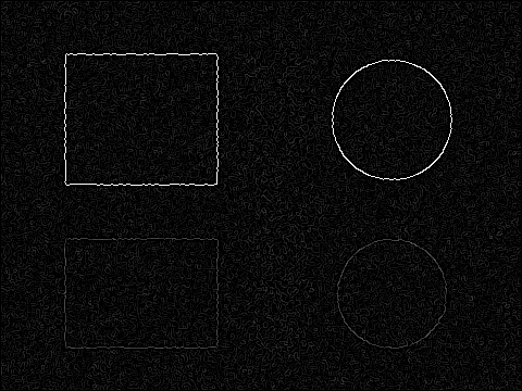
Step 2: Gradient computation. Apply Sobel to the smoothed image to obtain the magnitude \(A\) and direction \(\theta\) (Figure 13.5 (a)). Note that the strong contours are now bright bands several pixels wide — smoothing has spread the step out, and the gradient peak has widened with it.
Step 3: Non-maximum suppression (NMS). The gradient magnitude forms a ridge in the direction perpendicular to the edge, and the true edge should lie only on the ridge line. NMS works as follows: quantize each pixel’s gradient direction into 4 sectors (horizontal, 45°, vertical, 135°), compare the magnitude with one neighbor on each side along the gradient direction, and keep the center only if it is no smaller than one side and strictly greater than the other; otherwise set it to zero. The asymmetry of the comparison (\(\ge\) on one side, \(>\) on the other) is deliberate: when a flat plateau appears at the ridge top, only one side is kept, guaranteeing that the thinned result is single-pixel. In Figure 13.5 (b), the bands several pixels wide have been pared down to a thin ridge — but the local maxima of the noise have survived just the same; NMS handles “thin,” not “true.”
Step 4: Hysteresis thresholding with two thresholds. Separating edges from noise with a single threshold is doomed to sacrifice one side or the other, so Canny uses two: pixels with magnitude \(\ge\) the high threshold are seeds — strong enough to be trusted as edges; pixels with magnitude between the low and high thresholds are candidates — insufficient evidence on their own, but if 8-connected to a seed, they are accepted as the continuation of an edge. The implementation performs region growing from all seeds, expanding into every connected pixel whose magnitude is \(\ge\) the low threshold. The intuition is clear: a weak response hugging a strong edge is most likely the part of the same edge where the contrast fades; an isolated weak response is most likely noise. The strong vouch and the weak follow — only this way can a contour whose contrast waxes and wanes be preserved complete and connected.
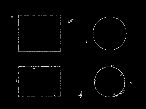
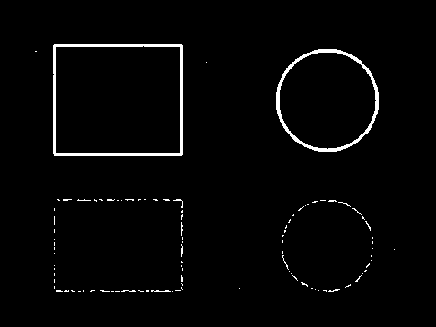
The final result, Figure 13.5 (c), contains 2163 edge pixels: the contours of all four shapes are fully preserved, single-pixel wide, and almost completely connected, with even the low-contrast rectangle and circle closing up intact. As a control, skipping NMS and hysteresis linking and binarizing the gradient magnitude directly with a single threshold (the same value, 60) yields Figure 13.6: 4064 edge pixels, nearly twice as many. Every extra pixel is waste — the strong contours become coarse bands 2–4 px thick (the gradient peak has width, and a single threshold scoops in the entire peak top), while the weak contours shatter into broken dashed lines (the magnitude oscillates about the threshold; what crosses stays, what doesn’t breaks). An edge map of uneven thickness and intermittent gaps is terrible input for downstream contour tracing and geometric fitting; NMS cures the “coarse,” hysteresis linking cures the “broken” — and that is precisely the respective value of Canny’s last two steps.
13.4 Choosing the Thresholds in Practice
Canny turned one threshold into two, and the responsibility of choosing them doubled as well. Both directions of failure are worth seeing with your own eyes (Figure 13.7).
Lowering the threshold pair to (8, 24) yields Figure 13.7 (a): 64077 edge pixels — 30 times the correct result. The gradient responses of the noise cross the low threshold en masse, then chain to one another through hysteresis linking, turning the whole image into a dense web; the sinusoidal grid of the central texture band also materializes in full. There is a design detail here worth spelling out: this scene’s texture has amplitude ±5 and period 12 px, and its gradient-magnitude peak measures about 19 — pressed just below the default low threshold of 20. That is why the texture region is spotless in the (20, 60) result, while under (8, 24) it floods out together with the noise. On real production lines, brushed, sandblasted, and woven surfaces all play the role of this texture band: whether they count as “edges” depends entirely on where you draw your threshold.
In the opposite direction, raising the threshold pair to (40, 120) yields Figure 13.7 (b): only 918 edge pixels remain, and the image is immaculately clean — but the low-contrast rectangle and circle have vanished entirely. After smoothing, the gradient magnitude of a contrast-20 edge falls short of 120; not a single seed can be produced, and hysteresis linking cannot make bricks without straw. In detection tasks, a miss is usually deadlier than a false alarm: false alarms can still be salvaged by downstream screening, but a missed target never comes back.
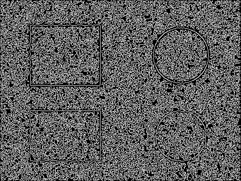
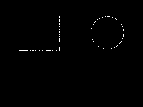
The engineering rule of thumb boils down to two steps. Step one, fix the high threshold: take 3–4 times the noise gradient level. Measure the typical level of the gradient magnitude in a blank region of the image (e.g. mean plus three standard deviations, or a high quantile) and anchor the high threshold at 3–4 times it — this guarantees that seeds almost cannot be produced by noise. Step two, fix the low threshold: start from 1/2 to 1/3 of the high threshold. The low threshold governs contour connectivity: too close to the high threshold and hysteresis linking exists in name only; too low and the noise builds bridges. This chapter’s (20, 60) was chosen exactly by this rule: after smoothing, the \(\sigma=8\) noise has a gradient magnitude of roughly 15, the high threshold of 60 is about 4 times that, and the low threshold is 1/3 of the high. Finally, fine-tune online with real images — the rule gives the starting point, not the destination.
This is kin in spirit to the histogram-based threshold selection of Chapter 7: there we thresholded the gray-value distribution to separate foreground from background; here we threshold the gradient-magnitude distribution to separate edges from noise. The object changed; the methodology of “look at the distribution, find the divide” did not.
13.5 Subpixel and Outlook
The edge pixels Canny outputs have only integer coordinates, nailing the localization precision to 1 px. For recognition and counting this is enough; for measurement it is nowhere near — in a system at 10 μm/px, 1 px of quantization error is 10 μm. Fortunately the remedy is cheap: NMS compares precisely the three magnitudes along the gradient direction, \(g_{-1}, g_0, g_{+1}\), and a parabolic interpolation over them pins the ridge-top position down to subpixel accuracy — the very same vertex formula that Chapter 14 used on one-dimensional profiles. Interpolating point by point along the contour upgrades the pixel chain to a subpixel contour. In industrial practice, if only a local edge or hole needs measuring, the more common tool is the caliper of Chapter 20, doing one-dimensional subpixel localization directly inside an ROI; whole-image edge detection is for the situations where you do not know in advance where the target is.
The SciVision SDK also offers a class of subpixel extractors complementary to Canny: SciSvExtractLinesGauss, which implements Steger-style curvilinear-structure detection (Steger 1998). Note that what it finds are not step edges but lines — ridges or valleys with width, such as scratches, bonding wires, or adhesive tracks. Based on Gaussian derivatives, ExtractLinesGauss directly outputs an array of center-line contours at subpixel accuracy, attaching attributes to each line: direction angle, response strength response, left/right half-widths, asymmetry, and contrast. Its parameters carry familiar shadows: sigma is the detection scale, and lowThresh/highThresh are the hysteresis threshold pair — the same idea as in Canny; lineModel selects among three profile models: Gaussian line, bar line, and parabolic. The companion CalculateParameter can even derive sigma and the two thresholds from the expected line width and contrast, sparing manual tuning. This chapter ran no experiment on it and offers it only as a pointer: when your target is “a line with width” rather than “a gray-value step,” this is the tool to remember.
13.6 SciVision Implementation
The operators used in this chapter are provided by SCIMV::SciSvFilter:
SCIMV::SciSvFilter f;
SciImage amp, lap, smooth;
SciROI roi;
SciPoint tl(0, 0), br(W, H); // GenRect1 bottom-right is an exclusive endpoint: pass (W, H) for the full image
roi.GenRect1(tl, br);
// Sobel gradient magnitude: sobelType=SUM_SQRT(1) is sqrt(gx^2+gy^2); kernelSize=3 (size of the Gaussian pre-smoothing kernel)
long rc = f.SobelAmplitude(img, roi, &, SCIMV::SUM_SQRT, 3);
// Laplace: 3x3 kernel, filterMask=1 (8-neighborhood kernel), resultType=0 (absolute-value output)
rc = f.Laplace(img, roi, &lap, 3, 1, 0);
// Canny pre-smoothing: 3x3 Gaussian, sigma=0.8
rc = f.Gaussian(img, roi, &smooth, 3, 3, 0.8, 0.8);SobelAmplitude’s sobelType selects how the magnitude is combined, SUM_SQRT being the standard square root of the sum of squares; kernelSize=3 is the size of the internal Gaussian pre-smoothing kernel (valid range [1,11]) and has nothing to do with the size of the Sobel derivative kernel. Laplace’s filterMask=1 selects the 8-neighborhood kernel (center \(-8\)), and resultType=0 outputs the absolute value — the double response of Figure 13.4 stems precisely from this.
The SDK also has a one-shot Canny(srcImage, ROI, dstImage) — but it has no threshold parameters whatsoever; the low and high thresholds are entirely built in, cannot be tuned per scene, and naturally cannot perform the sensitivity experiment of Section 13.4. This chapter therefore hand-wrote NMS and hysteresis linking (full code in the example project) — which happens to be the part most worth writing once with your own hands. If production code needs a Canny with controllable thresholds, the same advice applies: own these two steps yourself, leave the gradient and the smoothing to the SDK, and keep the decision logic in your own hands.
There is also a pitfall that must be recorded honestly: in the current version, SciSvFilter::Gaussian corrupts the rightmost 1–2 columns of the output image no matter what ROI is passed (with a kernel of 3, the last 2 columns are zeroed). The zeroed columns form a false step of contrast above 80 against their neighbors, showing up in the edge map as a false edge running the full image height. The example project’s countermeasure is to repair by replicating the last valid column to the right:
// SDK defect workaround: Gaussian zeroes the rightmost 2 output columns; fill them by copying the last valid column
for (int r = 0; r < H; ++r) {
    smooth[r * W + W - 2] = smooth[r * W + W - 3];
    smooth[r * W + W - 1] = smooth[r * W + W - 3];
}
The complete runnable project that generates all of this chapter’s images and statistics is located at code/edge_detection/; all edge-pixel counts (4064 / 2163 / 64077 / 918) are actual program output.
Industry Case: Threshold Tuning for Glass Edge-Chip Detection
A glass deep-processing line used Canny to extract the edge contour, then inspected the contour for local gaps to flag edge chips. The low and high thresholds were tuned against the images available at installation acceptance and then frozen. Months later, the night shift’s miss rate climbed: LED lumen decay compounded by lower ambient light at night reduced image contrast, the gradient magnitudes of small, faint chips fell below the frozen high threshold, and no seeds could be produced. The fix was per-shift automatic tuning: at the start of each shift, estimate the noise gradient level in a blank region beside the edge (a high quantile of the gradient magnitude), set the high threshold \(=K\times\) that estimate (\(K\approx 3.5\)), and the low threshold to half the high. Through several rounds of lamp aging and replacement since, the miss rate has held steady. The lesson: a gradient threshold measures “how much stronger the signal is than the noise”; a fixed absolute value silently decays along with the illumination — anchor the threshold to the noise, not to one day’s good lighting.
13.7 Summary
- Edges are gray-value discontinuities, characterized by the gradient: Sobel approximates the gradient with a pair of \(3\times 3\) kernels that “difference in one direction, smooth in the perpendicular one”; the magnitude decides “how strong,” the direction decides “which way.” The edge response is proportional to contrast — the root of every thresholding problem.
- Second-order operators are theoretically elegant, practically fragile: under \(\sigma=8\) noise, Laplace’s zero-crossing localization degenerates into a screenful of grain plus double-line responses, and it provides no directional information — industrial edge detection is dominated by first-order operators.
- Canny’s four steps each do one job: Gaussian smoothing resists noise, the gradient computes “likelihood,” NMS pares the response band down to a single-pixel thin ridge, and hysteresis thresholding — the strong vouch, the weak follow — preserves connected contours whose contrast waxes and wanes. In the experiments, single-threshold binarization at the same threshold output 4064 px of coarse, broken edges, while Canny output 2163 px of single-pixel connected contours.
- Anchor the thresholds to the noise: set the high threshold at 3–4 times the noise gradient level, start the low threshold at 1/2–1/3 of the high, then fine-tune online. In this chapter’s experiments, (8, 24) let noise and texture drown the result (64077 px), and (40, 120) wiped out the weak contours entirely (918 px).
- Measurement demands subpixel: parabolic interpolation over NMS’s three magnitudes yields subpixel edges; for line-like structures (scratches, bonding wires), the Steger-style
ExtractLinesGaussdirectly extracts subpixel center lines together with attributes such as width and contrast.
Two foundational papers reward a return to the originals: Canny’s classic derivation of this chapter’s four-step method from optimality criteria (Canny 1986), and Marr and Hildreth’s work laying the theoretical basis for second-order zero-crossing (LoG) detection (Marr and Hildreth 1980). For a systematic treatment of subpixel edge and line extraction, detection-scale selection, and their accuracy analysis, see the book by Steger et al. (Steger, Ulrich, and Wiedemann 2018).