31 Stereo Vision

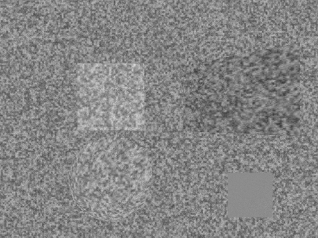
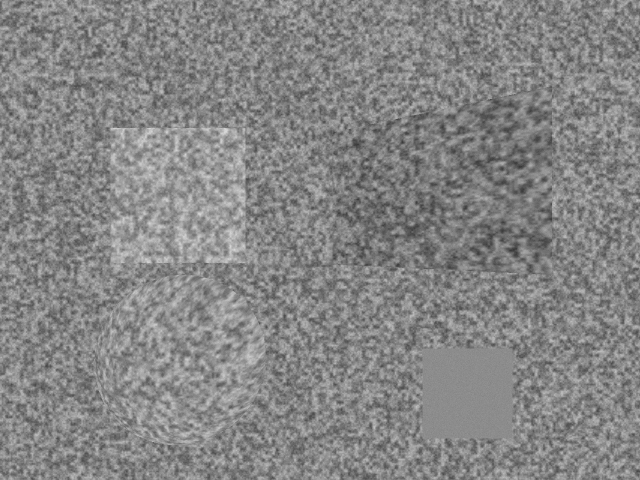
Humans have two eyes, and so we can tell at a glance which object is closer — the brain converts the tiny positional difference of the same target on the two retinas into distance. Machine vision can borrow this mechanism wholesale: shoot with two cameras separated by a certain distance at the same time, and the same spatial point lands at different horizontal positions in the two images; this positional difference is the disparity, and disparity directly encodes depth. Binocular stereo vision is the technique of inferring the depth of every pixel from a pair of images. Among the several 3D imaging routes listed in Chapter 30, it is the one closest to the human eye and also the most “passive”: it projects no energy onto the scene and relies only on ambient light, hence low power, no mutual interference, and the ability to work at long range. The price is an inescapable prerequisite — the measured surface must carry texture of its own, because finding disparity is essentially finding the correspondence of the same patch of pattern across the two images, and without texture there is nothing to correspond. This chapter starts from epipolar geometry, proceeds through block matching, reliability checking, subpixel refinement and windowing, and finally arrives at depth reconstruction, throughout using one synthetic rectified stereo pair (Figure 31.1).

31.1 Epipolar Geometry and Disparity

When two cameras look at the same point, the geometry is not entirely unconstrained. The spatial point and the two camera optical centers jointly determine a plane, which intersects the two image planes in a pair of epipolar lines — this is the core conclusion of epipolar geometry: the corresponding point in the right image of a given pixel in the left image must lie on its corresponding epipolar line, rather than roaming all over the image. This reduces a two-dimensional search to a one-dimensional one. Engineering goes one step further: through rectification a projective transform is applied to the two images so that all epipolar lines are strictly parallel to the image rows and their row indices align one-to-one. After rectification, the corresponding point of a pixel on row \(y\) of the left image must lie on the same row \(y\) of the right image, offset only in the \(x\) direction. This is exactly the state of this chapter’s stereo pair: finding correspondence degenerates into a one-dimensional slide along the same row.

This example’s stereo pair is already in the rectified state at the synthesis stage (the two cameras differ only by a translation along \(X\) and share identical intrinsics), so in-row search can be done directly. A real system must first perform the binocular calibration of Chapter 5, solving for the relative pose and distortion of the two cameras, and then compute the rectification mapping accordingly — rectification quality directly decides the success or failure of subsequent matching: even half a pixel of residual vertical misalignment makes block matching systematically worse.

Let the two camera optical axes be parallel, separated by the baseline \(B\), with focal length \(f\) (in pixels); for a point at depth \(Z\), the difference in horizontal coordinate between the left and right images is the disparity \(d\). From similar triangles we get \(d/f = B/Z\), that is

\[ Z = \frac{fB}{d}. \tag{31.1}\]

Disparity is inversely proportional to depth: the nearer the object the larger the disparity, the farther the smaller. In this example \(f=600\) px and \(B=60\) mm, so \(fB=36000\) mm·px, and the ground-truth disparity falls within 36.0–51.4 px (corresponding to \(Z\) from 1000 mm to 700 mm). In Figure 31.1 the near objects shift left noticeably while the background barely moves, which is exactly the intuitive manifestation of this inverse relationship.

The inverse relationship also has a far-reaching corollary. Differentiating Equation 31.1 gives the depth error corresponding to one pixel of disparity error, namely the depth resolution

\[ \Delta Z = \frac{Z^2}{fB}. \tag{31.2}\]

It grows with \(Z^2\) — this is the mathematical essence of “stereo is less accurate farther away.” In this example at \(Z=1000\) mm, each 1 px of disparity corresponds to 27.8 mm of depth; while at \(Z=800\) mm it is only 17.8 mm, and at \(Z=700\) mm it drops further to 13.6 mm. The same disparity measurement error gets amplified into several times the depth error at a distance. This formula also points to two directions for improving accuracy: increase \(fB\) (longer focal length or longer baseline), or measure disparity to subpixel accuracy — the latter being the subject of Section 31.4.

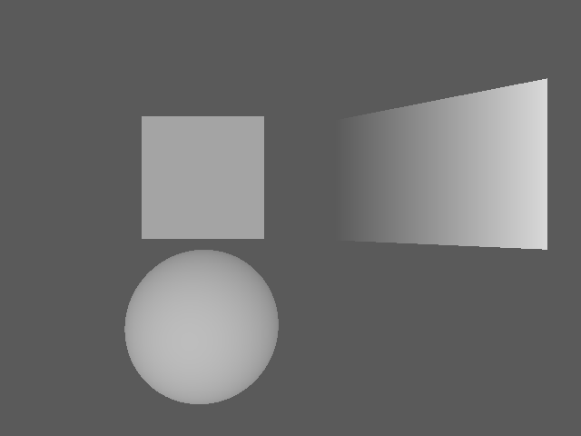
Figure 31.2 is the ground-truth disparity field of this scene (obtained per pixel from the known depth via Equation 31.1), and all subsequent matching results will be measured against it. Note that the box and spherical cap (near objects) are brighter overall (large disparity), the background is darker (small disparity), and the ramp shows a continuous gradient from near to far — this is exactly the pictorial presentation of the inverse relationship in Equation 31.1, and also the target that block matching ought to approach.

Figure 31.2: Ground-truth disparity field back-computed from the known depth (bright = large disparity = near). It is the yardstick for evaluating all subsequent matching results: the box/spherical cap are bright, the background is dark, and the ramp is a continuous gradient.

The baseline \(B\) is a typical trade-off quantity. By Equation 31.2, the longer the baseline the higher the depth resolution; but the longer the baseline, the larger the viewpoint difference between the two cameras, and the larger the occlusion regions blocked by the foreground and visible to only one eye, while the same surface suffers more severe perspective deformation across the two images and is harder to match. The baseline choice of an industrial stereo rig must compromise between “accuracy” and “occlusion / matching difficulty,” and is usually set to some fraction of the working distance.

31.2 Block Matching

After rectification, finding disparity is simply: for each pixel of the left image, slide along the same row of the right image and find the most similar position. “Similar” needs a cost function. The most naive is the sum of absolute differences (SAD) — take a small window centered on the pixel, compute the absolute difference of left-right gray values point by point and sum them; the smaller the cost the more alike. This is of the same origin as the template matching of Chapter 16, only the template is replaced by “a local window of the left image” and the search range is constrained by epipolar geometry to within one row. More robust to illumination changes is normalized cross-correlation (NCC), but it is heavier to compute. This example uses SAD and restricts the search to the disparity interval \([30, 56]\) px (derived from the scene’s known depth range plus margin).

Computing the window cost for every pixel and every candidate disparity yields a three-dimensional cost volume \(C(x,y,d)\). Taking the position of minimum cost along the \(d\) dimension gives the integer disparity of that pixel — this step is called “winner-take-all.” Figure 31.3 is the raw integer disparity result of an 11×11 window: the shapes of the box, ramp, and spherical cap all emerge correctly, near objects bright (large disparity), background dark (small disparity). But look closely at the ramp and the spherical cap and you find obvious quantization banding — depth that ought to transition smoothly is cut into a staircase, exactly the discretization trace of integer disparity: the true disparity is a continuous fraction, while winner-take-all can only output integers.

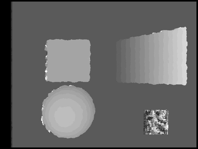
Figure 31.3: Raw integer disparity of 11×11 SAD block matching (near objects bright, far dark). Staircase quantization banding is visible on the ramp and spherical cap, a direct consequence of integer disparity discretization; the textureless patch at the lower right shows chaotic random disparity.

Quantitatively, this 11×11 SAD reaches 91.8% valid rate over the whole image, mean absolute error (MAE) of 0.362 px, and a bad-pixel rate (error > 1 px) of 3.93%. If we count only non-occluded regions, the MAE drops to 0.299 px — confirming that one major source of error is occlusion: background pixels blocked by the foreground simply have no correspondence in the right image, and winner-take-all can only assign them a wrong minimum-cost match. In this example the ground-truth occlusion accounts for 0.92%, concentrated in the background band along the left edge of near objects. How to identify these unreliable disparities is the task of the next section.

31.3 Failure and Reliability

Winner-take-all will always give a “best” disparity, even where the region has no reliable correspondence at all. A naive yet effective discrimination means is the left-right consistency check: compute a disparity map \(d_L\) with the left image as reference, then compute another \(d_R\) with the right image as reference, and cross-check — if the disparity of left-image pixel \(x\) is \(d_L(x)\), its corresponding point in the right image is \(x-d_L\), then \(d_R(x-d_L)\) should be almost equal to \(d_L(x)\). Pixels where the two disagree (threshold taken as 1 px in this example) are judged unreliable and discarded. Occlusion regions are naturally caught by this check: the “corresponding point” of an occluded pixel actually belongs to the foreground, the two matches each tell their own story, and they are bound to disagree.

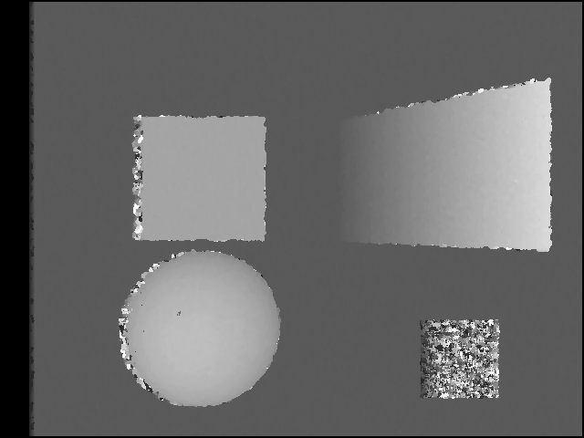
Figure 31.4 is the disparity map after checking: most of the occlusion band (left edge of near objects) and the textureless patch have been culled to black (invalid), and the retained disparities are cleaner. The price is that the whole-image valid rate drops from 91.8% to 88.6%, but the quality of the retained pixels improves substantially — MAE improves from 0.362 px to 0.134 px, and the bad-pixel rate is squeezed from 3.93% down to 1.26%. The reliability check does not create accuracy; it merely honestly marks out the places where “I don’t know,” which in industry is often far more useful than a seemingly dense but actually adulterated disparity map.

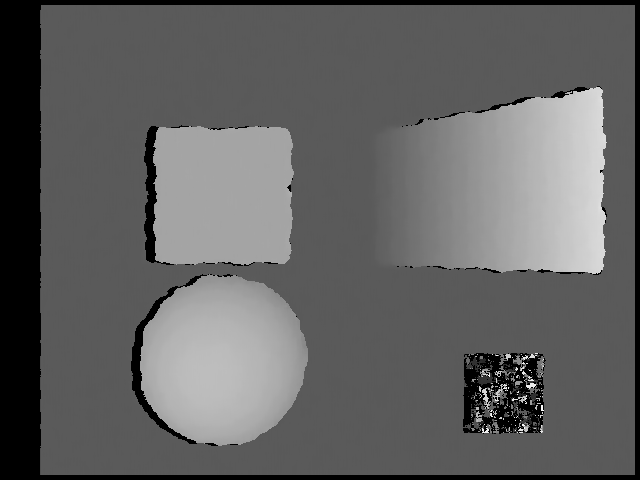
Figure 31.4: Disparity map after the left-right consistency check. The occlusion band and textureless patch are culled to black (invalid); the MAE of the retained pixels drops from 0.362 px to 0.134 px. Honestly marking out the regions that “cannot be reliably measured” is a key step toward making stereo vision engineering-usable.

The most illustrative case is the 90×90 px textureless patch at the lower right corner — it is a deliberately designed failure region. In Figure 31.3 it shows a mess of random disparity, and the raw statistics reveal: this region has a raw valid rate as high as 100%, yet 82.2% of it is bad pixels. The reason is simple: every position on a uniform gray patch looks identical, the SAD cost curve is nearly flat across the entire search range, and the “minimum” picked by winner-take-all is determined purely by sensor noise — a thoroughly random solution. Even more telling is what happens after the left-right check: only 43.3% of the pixels of the textureless patch survive, and among the survivors still 82.5% are bad pixels. In other words, even when two random matches “happen” to agree, what they agree on is still wrong — no texture, no stereo.

The lesson of the textureless patch directly explains the motivation of actively projecting texture in Chapter 32: since passive stereo is helpless on textureless surfaces, then actively project a sheet of artificial random speckle or coded fringes onto the scene, manufacturing texture available for matching. This is also the core idea of “active stereo” sensors — the geometric framework of stereo is unchanged, only a projector supplies the prerequisite of texture.

31.4 Subpixel and Windowing

The quantization banding of integer disparity (Figure 31.3) comes from winner-take-all being able to take only integers. The remedy is just like the subpixel edge localization in Chapter 14 and Chapter 20: at the integer disparity \(d_0\) of minimum cost, take the three cost values \(C_{-1},C_0,C_{+1}\) of it and its left and right neighbors \(d_0\pm1\) and do parabolic interpolation; the offset of the parabola vertex relative to \(d_0\) is

\[ \delta = \frac{C_{-1}-C_{+1}}{2\,(C_{-1}-2C_0+C_{+1})}, \tag{31.3}\]

and the subpixel disparity is \(d_0+\delta\). Three samples determine one parabola, the vertex formula is closed-form, and the computational cost is negligible — once again, accuracy almost for free. The effect is most intuitive in the ramp region (where the true value is a continuous fractional disparity): there the integer-disparity MAE is 0.252 px, and after subpixel interpolation it plunges to 0.070 px. The whole-image non-occluded error histogram also moves accordingly: the fraction of pixels with \(|\text{err}|\le 0.125\) px rises from 80.4% for integer to 91.6% for subpixel. The whole-image MAE improves from 0.362 to 0.342 px, and the non-occluded one from 0.299 to 0.278 — the quantization banding is smoothed away.

Another knob that must be tuned to the scene is the window size. A large window admits more texture and averages noise more fully, but it presumes that “the entire window belongs to one depth,” and at depth discontinuities (object edges) it smears foreground and background together. The table below contrasts three window sizes — 5×5, 11×11, 21×21 — in the non-occluded region (subpixel disparity):

Table 31.1: Window size trade-off: a large window is more accurate overall but worsens at edges (non-occluded, subpixel disparity)

Window	MAE (px)	Bad-pixel rate	Edge-ring bad pixels	Textureless bad pixels
5×5	0.336	3.69%	3.95%	90.5%
11×11	0.278	3.38%	4.26%	86.7%
21×21	0.251	3.24%	5.17%	65.5%

Read this table region by region. The overall MAE decreases as the window grows (0.336 → 0.251), because a large window suppresses noise more aggressively; but the bad-pixel rate of the edge ring (12 px on each side of the box boundary) worsens in the opposite direction (3.95% → 5.17%) — this is edge bleeding: a large window also counts background pixels outside the foreground edge, so the edge is “fattened” by the foreground. Figure 31.5 contrasts the two extremes 5×5 and 21×21: win5 is noisier with sharp edges, win21 is smooth and clean but the contours of the box and ramp are clearly swollen. Interestingly, the textureless bad-pixel rate drops from 90.5% for win5 to 65.5% — the large window borrows the externally adjacent texture in too, scraping together a bit of matchable content for the otherwise hopeless gray patch, but this is borrowed and not trustworthy.

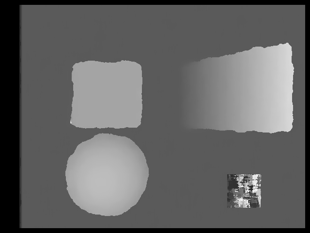
Edge bleeding can be quantified to the specific pixel. Measuring the disparity-crossing position of the box edge on row \(y=195\): the box left edge has true value \(x=155\), and the three windows measure 148/151/152 — the larger the window the more it biases to the outer left (foreground expansion); the right edge has true value \(x=290\), measured 291/292/293 — likewise swelling outward. Each step up in window size expands the foreground edge by roughly half a window width. This explains why industry often places extra distrust on the disparity near foreground edges, or simply switches to algorithms with adaptive windows or global smoothness constraints.

31.5 Depth Reconstruction

With a reliable disparity map, applying Equation 31.1 per pixel as \(Z=fB/d\) gives the depth map (Figure 31.6). This map is essentially a 2.5D range image — it records the distance to the nearest surface in each pixel direction as seen from the camera, rather than a complete three-dimensional model (no data for the back side or occluded places), consistent with the definition of 2.5D in Chapter 30. To go further and obtain metric 3D points, one still needs the camera intrinsics to back-project each \((x,y,Z)\) into \((X,Y,Z)\), which enters the point-cloud realm of Chapter 37.

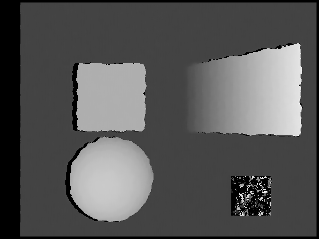
Figure 31.6: Depth map converted from the disparity map via \(Z=fB/d\) (near bright, far dark). This is a 2.5D range image: it records only the distance to the nearest surface in each line-of-sight direction. The reconstructed box height is 200.1 mm (true value 200).

In terms of accuracy, the measurement results are convincing: the background median depth is 1000.0 mm (true 1000), the box face is 800.0 mm (true 800), so the reconstructed box height is 200.1 mm, against a true value of 200 mm — an error of a few tenths of a millimeter. Here the subpixel dividend of Section 31.4 is exactly recovered: by Equation 31.2, the depth resolution at \(Z=1000\) mm is 27.8 mm/px, and with only integer disparity the depth would be nailed to a ~28 mm staircase, with no way to measure the 200 mm box height to one decimal place. But the 0.1 px subpixel accuracy raises the effective depth resolution to 2.78 mm (×10), and only then can the box height be pinned to 200.1 mm. Subpixel is not icing on the cake; it is the watershed of whether stereo can do metric measurement.

31.6 SciVision Implementation

It must be stated honestly: the SciVision SDK provides no binocular stereo matching library — there is no ready-made API for rectification, cost volume, disparity solving, or left-right checking. Therefore the companion project of this chapter code/stereo_vision/ is a self-contained C++ implementation, with the SDK used only for image I/O (SciImage::SaveImage outputs PNG). Below are three core code segments.

Winner-take-all over the cost volume (SAD accelerated by box filtering with integral images; the integral-image details are omitted here, illustrating only the optimal-disparity solve and subpixel):

int best = BIG, bi = -1;                  // find the minimum cost along the disparity dimension
for (int di = 0; di < ND; ++di) {
    int c = cost[((size_t)di * H + y) * W + x];
    if (c < best) { best = c; bi = di; }
}
m.id[i] = D0 + bi;  m.d[i] = (float)(D0 + bi);  m.valid[i] = 1;
if (bi > 0 && bi < ND - 1) {              // parabolic subpixel interpolation
    double cm = cost[((size_t)(bi-1)*H + y)*W + x];
    double cp = cost[((size_t)(bi+1)*H + y)*W + x];
    double denom = cm - 2.0 * best + cp;
    if (denom > 1e-9) {
        double offd = 0.5 * (cm - cp) / denom;   // i.e. eq. @eq-sv-subpix
        if (offd > 0.5) offd = 0.5; else if (offd < -0.5) offd = -0.5;
        m.d[i] = (float)(D0 + bi + offd);
    }
}

Left-right consistency check (cross-checking the left and right match results):

auto bmR = blockMatch(right, left, false, 11);   // match once more with the right image as reference
for (int y = 0; y < H; ++y)
    for (int x = 0; x < W; ++x) {
        int i = y * W + x;
        if (!bm11.valid[i]) continue;
        int xr = x - (int)std::lround(bm11.d[i]);     // corresponding point of the left-image pixel in the right image
        if (xr < 0 || xr >= W || !bmR.valid[y*W+xr]) continue;
        if (std::fabs((double)bm11.d[i] - bmR.d[y*W+xr]) <= 1.0)  // keep only if consistent
            lrValid[i] = 1;
    }

blockMatch(left, right, true, 11) and blockMatch(right, left, false, 11) solve \(d_L\) and \(d_R\) respectively, win=11 is the window edge length, and D0=30, D1=56 frame the search interval. This pattern of “the algorithm living outside the SDK” is no accident: industrial stereo is extremely sensitive to compute and latency, and real products mostly push stereo matching down into a dedicated sensor or FPGA — disparity solving is a regular, massively parallelizable per-pixel operation, naturally suited to a hardware pipeline, and belongs to a different layer than the “call-the-library” paradigm of a general CV SDK. The place for a library like SciVision is after the disparity/depth map is produced: use its filtering, morphology, blob, and measurement tools to process the depth map and complete downstream tasks such as sizing and defect inspection.

Industry Case: Texture Dependence in Logistics Sorting

Logistics sorting lines often use stereo cameras to measure parcel volume (length, width, height) online, for billing and packing planning. In practice success or failure depends almost entirely on surface texture: a kraft cardboard box has printing, tape, and fiber texture on its surface, the disparity is dense and reliable, and the volume is measured fast and accurately; but the moment you encounter a black plastic bag, reflective sealing tape, or specular packaging, the surface is either textureless or the specular reflection breaks the Lambertian assumption, and the disparity fails over large areas — the measured volume is either incomplete or jumps around. There are two countermeasures: one is to switch to active stereo, adding projected speckle to artificially create texture on the surface (echoing Chapter 32); the other is multimodal hole-filling, using time-of-flight or structured light to patch where stereo fails. The lesson is direct: the prerequisite of passive stereo is that “the measured surface carries texture of its own,” so before going live always verify the texture characteristics of the target surface, then decide whether to use passive stereo, active stereo, or switch to a different technology route.

31.7 Summary

Disparity is depth: epipolar geometry constrains the correspondence search to one epipolar line, which degenerates after rectification into a one-dimensional in-row search; depth is given by \(Z=fB/d\), and disparity is inversely proportional to depth.
Depth resolution worsens with \(Z^2\) (\(\Delta Z=Z^2/(fB)\)): in this example 27.8 mm/px at 1000 mm, and being less accurate farther away is an intrinsic limitation of stereo, mitigated by increasing \(fB\) or by subpixel.
Block matching + winner-take-all gives integer disparity (11×11 SAD: MAE 0.362 px), but integer quantization produces staircase banding; parabolic subpixel interpolation smooths the banding almost for free, dropping the ramp-region MAE from 0.252 to 0.070 px and raising the effective depth resolution from 27.8 mm to 2.78 mm — subpixel is the watershed of stereo doing metric measurement.
The left-right consistency check honestly culls occlusion and textureless regions (valid rate 91.8% → 88.6%, but retained-pixel MAE improves to 0.134 px); no texture, no stereo — the textureless patch is 100% valid raw yet 82% bad, and still 82.5% bad after checking, which is exactly the motivation of active texture-projection schemes such as structured light.
Window size is a dilemma between accuracy and edge fidelity: a large window is more accurate overall (MAE 0.251) yet makes the foreground edge bleed and swell (edge bad pixels 3.95% → 5.17%), with the box edge expanding outward by about half a window width per step, so engineering must compromise per scene or switch to adaptive/global methods.

For the classic treatment of epipolar and multi-view geometry, see the monograph by Hartley and Zisserman (Hartley and Zisserman 2004); the systematic taxonomy and evaluation of dense stereo matching costs and algorithms is given in the classic survey by Scharstein and Szeliski (Scharstein and Szeliski 2002), and semi-global matching (SGM), the industrial workhorse balancing accuracy and efficiency, was introduced by Hirschmüller (Hirschmüller 2008). The engineering realization and uncertainty analysis of stereo matching in industrial vision can be further consulted in the work of Steger et al. (Steger, Ulrich, and Wiedemann 2018).