17 Shape Matching
The previous chapter (Chapter 16) crowned NCC as the workhorse of industrial localization, and also exposed its boundaries at the end: NCC resists neither rotation nor occlusion, and it cannot hold the line against nonlinear illumination. On a production line these three regular visitors cross the boundary again and again — incoming parts arrive at random angles, grippers and carrier tapes cover part of the workpiece, and specular highlights and oil films warp the gray-value mapping into an arbitrary curve. All three failures share one root cause: gray-value matching compares the gray value of every single pixel, and gray values are precisely the least stable thing in an image — and the pixel patch itself is nailed to one orientation and one size. The way out is to change what we compare — not gray values, but shape: abstract the template into a set of edge points (position + gradient direction), search over a pose grid of angle and scale, and at each point check only whether the image’s gradient direction agrees. This is shape-based matching, the most interference-resistant localization algorithm in commercial vision libraries.
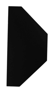
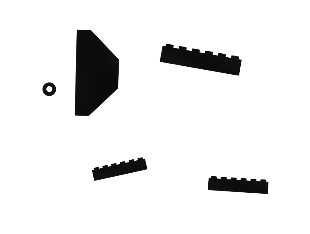
This chapter runs its experiments on a set of real industrial sample images. The contour-matching images come from a localization recipe’s silhouette samples (Figure 17.1): black parts on a white background, with the lead role played by a pentagonal wedge — a vertical left edge, a near-horizontal top edge, a tip converging to the right, and a chamfered corner at the lower right; the flat edges and the chamfer make it strongly non-rotationally-symmetric. The supporting cast includes a ring washer and a toothed rack as distractors. Across the five sample images the wedge is scattered at a wild variety of angles (Section 17.2), exactly testing rotation robustness and clutter rejection. The scale experiment uses a separate set: the same pile of parts (a screw, a knob, a square connector) photographed at three working distances, the parts shrinking from near to far as the camera pulls back (Section 17.4).
17.1 Similarity Based on Gradient Direction
The model in shape matching is not a pixel patch but a list of edge points: at training time, edge extraction is run on the template (the hysteresis-threshold pipeline of Chapter 13), yielding \(n\) edge points \(p_i\), each carrying the gradient direction \(\theta_i\) at that location. At search time the list is transformed onto the image under a candidate pose (translation + rotation + scale); at each point’s landing position the image’s gradient direction is read out and differenced against the model direction (rotated along with the pose) to give \(\Delta\theta_i\), and the score is the average direction agreement:
\[ s=\frac{1}{n}\sum_{i=1}^{n}\cos\Delta\theta_i . \]
When the directions agree perfectly, \(\cos\Delta\theta_i=1\) and \(s=1\) (which the SDK reports on a 100-point scale). When directions are random, positive and negative contributions cancel and tend to zero. Hidden inside this one formula are shape matching’s three great weapons.
Naturally searchable over rotation and scale, because the model is a list of points with geometric coordinates: rotate it by \(\phi\) and scale it by \(\sigma\) as a whole and you get the prediction for a new pose, so scoring pose by pose localizes across continuous angle and scale — exactly what a gray-value patch cannot do: a patch must be resampled the moment it rotates, and the NCC formula has no degree of freedom for angle in the first place.
Robust to illumination, because gradient direction does not change under gray-value gain and offset: replace the image with \(a f + b\) (\(a>0\)) and the gradient vector becomes \(a\nabla f\) — its length changes, but its direction does not budge. Better still, even when the gray-value mapping is nonlinear, as long as it is locally monotonic, the course of the iso-gray contours is unchanged and the direction is still conserved. NCC holds the line at linear; gradient direction holds it even for smooth nonlinearities.
When \(a<0\) (light–dark inversion), the gradient direction flips by \(180^\circ\) and \(\cos\Delta\theta_i=-1\) — the score is penalized instead. Whether to score by \(\cos\) (requiring consistent polarity) or by \(\lvert\cos\rvert\) (ignoring polarity) is controlled by the SDK’s polarity parameter: specular reflection on curved surfaces and backlight switching flip local polarity, and only then should it be opened up to 2.
Natural tolerance of occlusion, because the score is an average of per-point contributions: model points that land on the occluder see a gradient direction unrelated to the model, so their contributions are random within \([-1,1]\) with near-zero mean — missing points merely dilute the score without disturbing the contributions of the remaining visible points in the slightest. If 70% of the part is visible, roughly 70% of the score remains. Contrast NCC: occluded pixels enter the sum of squares at full weight, carrying enormous gray-value residuals, and a small amount of occlusion is enough to drag the correlation beyond recognition. One is “majority rules,” the other is “one vote vetoes” — and that is where the gap in robustness comes from.
17.2 Rotation and Clutter Experiment
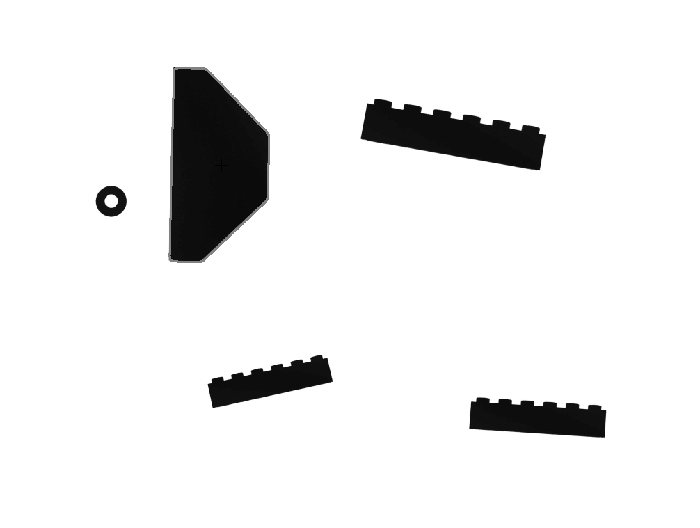
Build a model from the wedge in sample 1 with SciSvScaleShapeMatch (angle range \(\pm 180^\circ\), step \(1^\circ\), scale fixed at 1.0) and search the full image of all five samples with minScore = 40. Six wedges are scattered across the five images (sample 3 holds two in one frame), and all six are hit, with angles spanning from \(-152^\circ\) to \(+102^\circ\) — a full \(254^\circ\) range of rotation:
| Sample | Instance | Position (px) | Solved angle | Score |
|---|---|---|---|---|
| 1 | Wedge (template source, upright) | \((318, 237)\) | \(0^\circ\) | 99.8 |
| 2 | Wedge (large rotation) | \((455, 497)\) | \(-152^\circ\) | 99.8 |
| 3 | Wedge A | \((325, 196)\) | \(102^\circ\) | 99.6 |
| 3 | Wedge B | \((323, 570)\) | \(89^\circ\) | 93.7 |
| 4 | Wedge (near-upright) | \((702, 252)\) | \(1^\circ\) | 99.8 |
| 5 | Wedge (rotated) | \((310, 209)\) | \(-68^\circ\) | 95.5 |
Positions are pixel coordinates in the \(1006\times 759\) downsampled image. The SDK returns angles in the mathematically positive direction (counterclockwise positive); they are negated when rendering in image coordinates (\(y\) downward). The silhouette edges have extremely high contrast, so the hit scores across all five images stay above 93 no matter how large the rotation — a direct consequence of “comparing direction, not gray value.”
Two points are most worth savoring. First, none of the distractors is falsely detected: every image is given three slots (matchCount=3), yet the ring washer and toothed rack — parts with “the wrong shape” — never reach minScore=40. The gradient-direction list recognizes the wedge’s unique combination of edge segments; the washer’s arcs and the rack’s square teeth simply do not match. Second, the redrawn model contour fits precisely: the gray thin line on each wedge in Figure 17.2 is the model’s edges redrawn at the solved pose (including the rotation angle), wrapping the part’s true boundary tightly — even the one in sample 2, flipped by \(152^\circ\), is dead on.
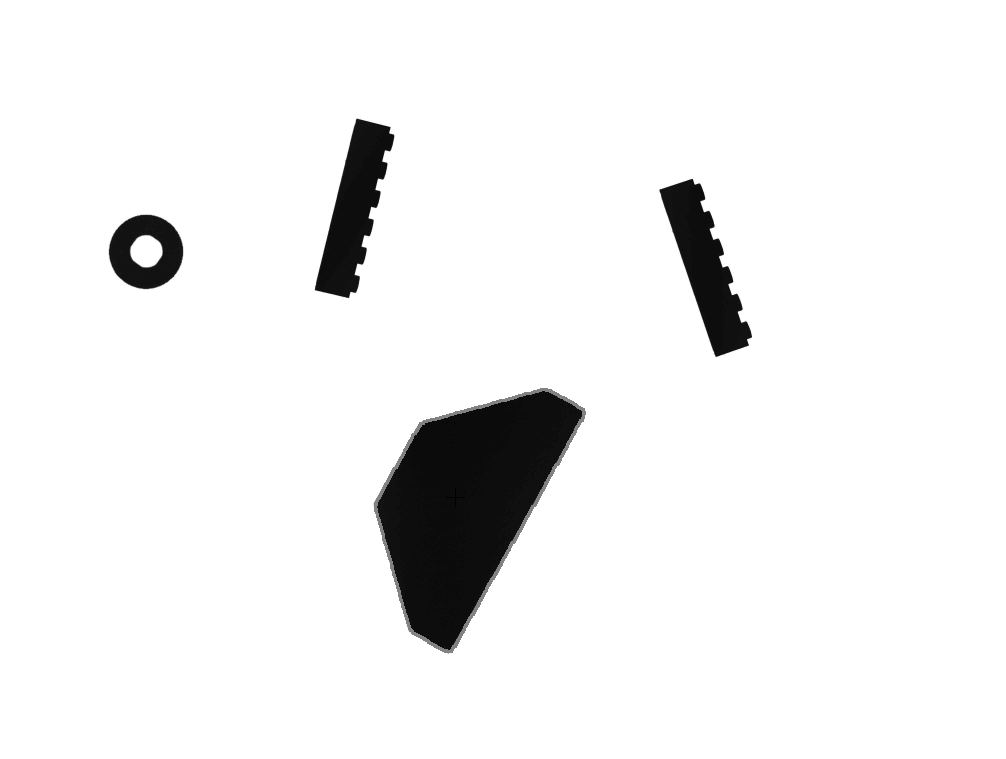
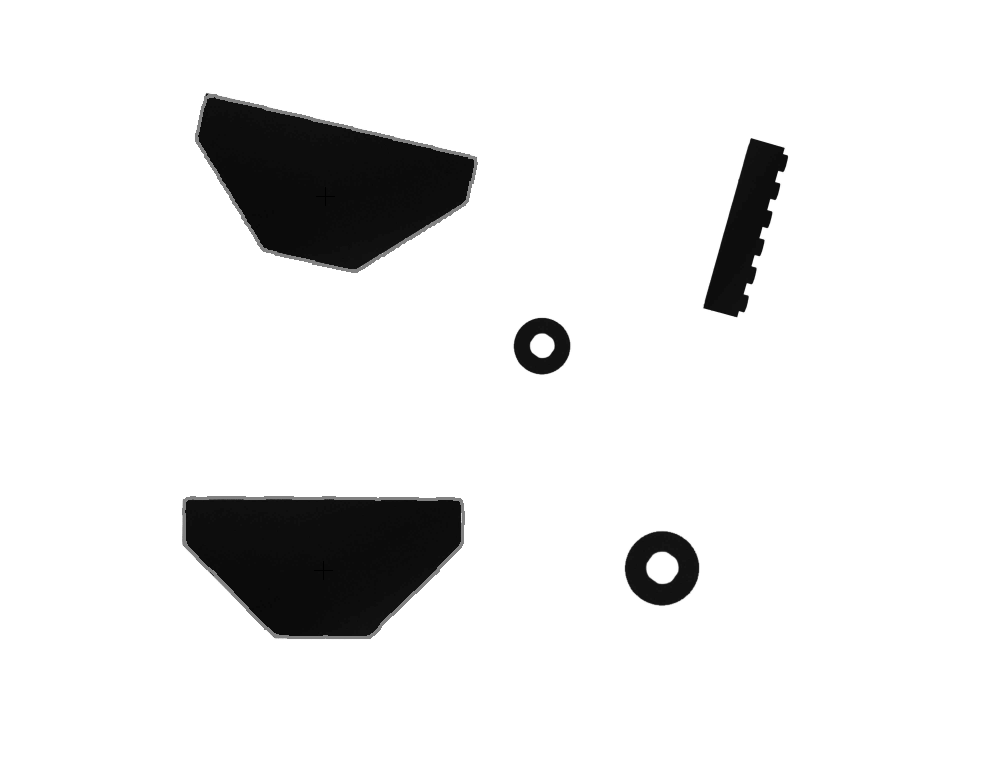
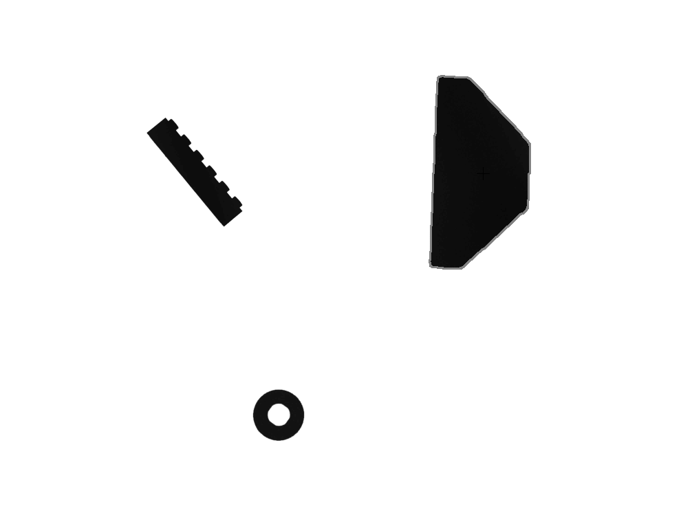
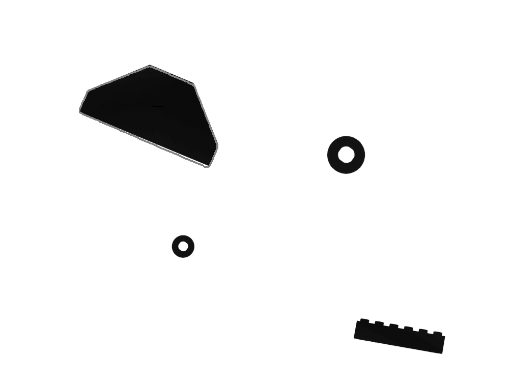
Drag grayscale NCC in to do the same job, and it is immediately exposed. Using the upright wedge template (with no rotation search whatsoever) to compute correlation: at the upright instance in sample 1 the NCC is 1.000 (the template was cropped from there), but at the center of that rotated instance in sample 2 (the position given by shape matching) the NCC plunges to 0.585 — far below the customary 0.80 decision line. NCC’s convolution window is nailed to one orientation, so the moment the workpiece turns it no longer aligns and the score collapses; shape matching makes angle an explicit search dimension and finds the part wherever it has turned. This is the most fundamental divide between NCC and shape matching: the former recognizes only one pose, the latter searches the entire pose space.
17.3 Occlusion Experiment
In the real samples the parts are well separated, with no ready-made occlusion scene, so a synthetic mid-gray occluding bar is overlaid on the wedge in sample 1 (simulating a carrier tape or gripper crossing the workpiece), with all other pixels kept real. The bar covers 36.0% of the part’s area (visible fraction 0.64). Searching again, shape matching still hits squarely: the pose locks at \((318, 237)\), \(0^\circ\) — identical to the un-occluded case — and the score drops from 99.8 to 76.5, a degradation ratio of 0.77, the same order as the visible fraction of 0.64. The “score ≈ visible fraction” of Section 17.1 holds up broadly in the commercial implementation; that it runs a touch above 0.64 is because the bar happens to cross the middle of the part, while the wedge’s directional features are more densely concentrated at the tip and the chamfer, which remain exposed.
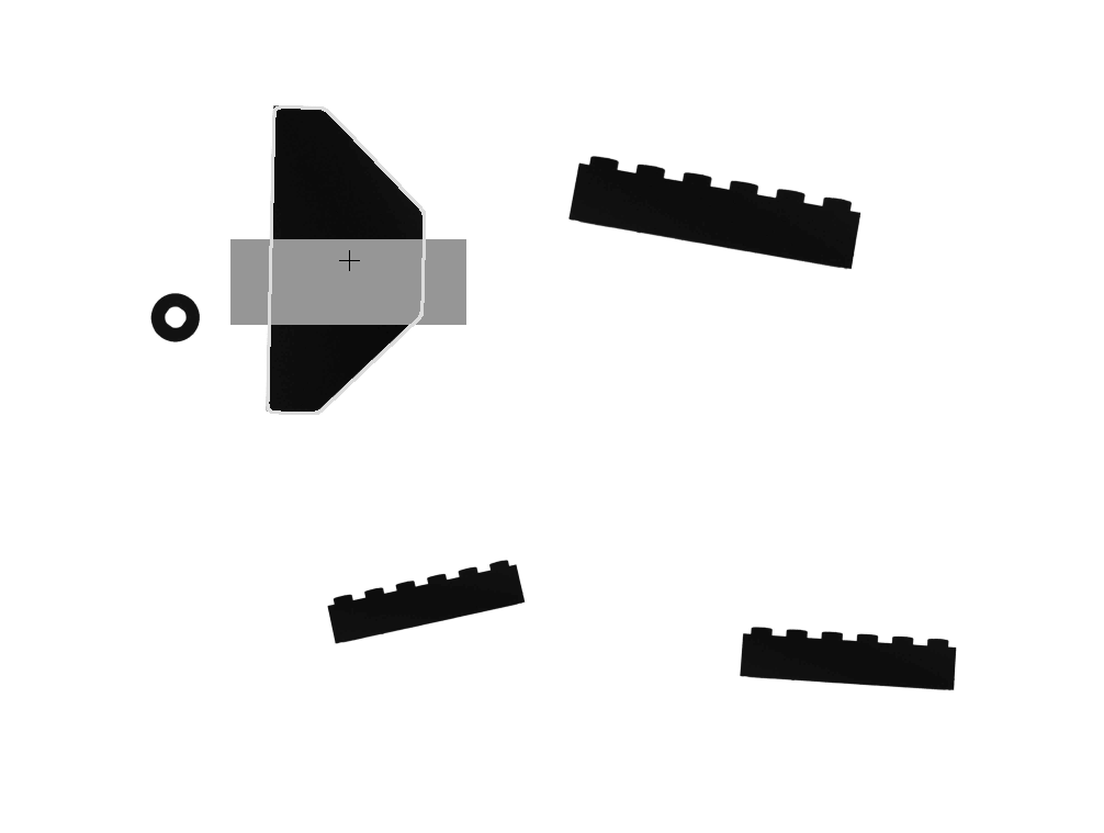
From this follows the engineering reading of minScore: it is the maximum occlusion fraction you are willing to tolerate. An intact wedge scores 95–100; setting minScore to 40 tacitly permits about 60% of the contour to be missing, while setting it to 70 demands an essentially complete part. But occlusion resistance is not determined by minScore alone: the coarse-screening parameter partialThreshold requires a sufficient fraction of the model to be visible at the coarse pyramid levels, and it must be opened up along with the occlusion budget (0.4 here) — otherwise the occluded candidate is eliminated at the coarse level and never reaches fine scoring.
17.4 Scale Matching
Localization has a fourth degree of freedom. Once the camera-to-workpiece distance changes — a model changeover, a different pallet height, a refocused lens — the part’s scale in the image changes, and a fixed-size template immediately fails to line up with the contour. The remedy is exactly as for angle: make scale an explicit search dimension too. At training time, poses are pre-generated on the angle × scale grid according to startScale/scaleExtent/scaleStep, and at search time every grid cell is scored.
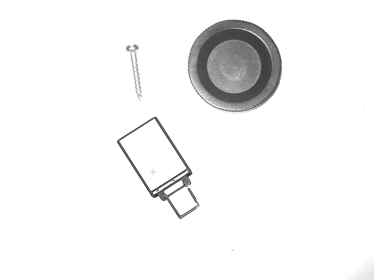
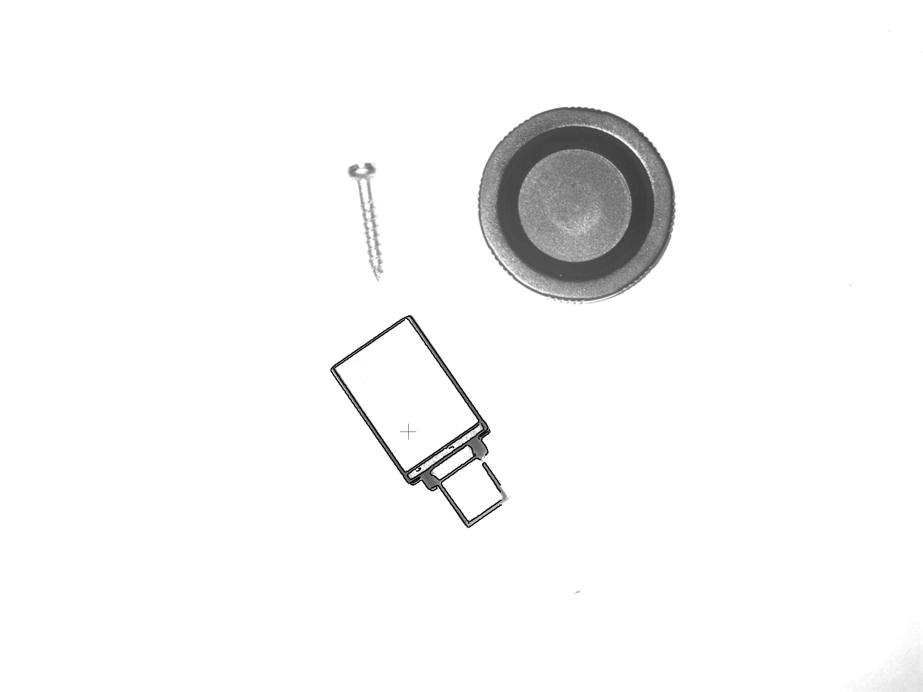
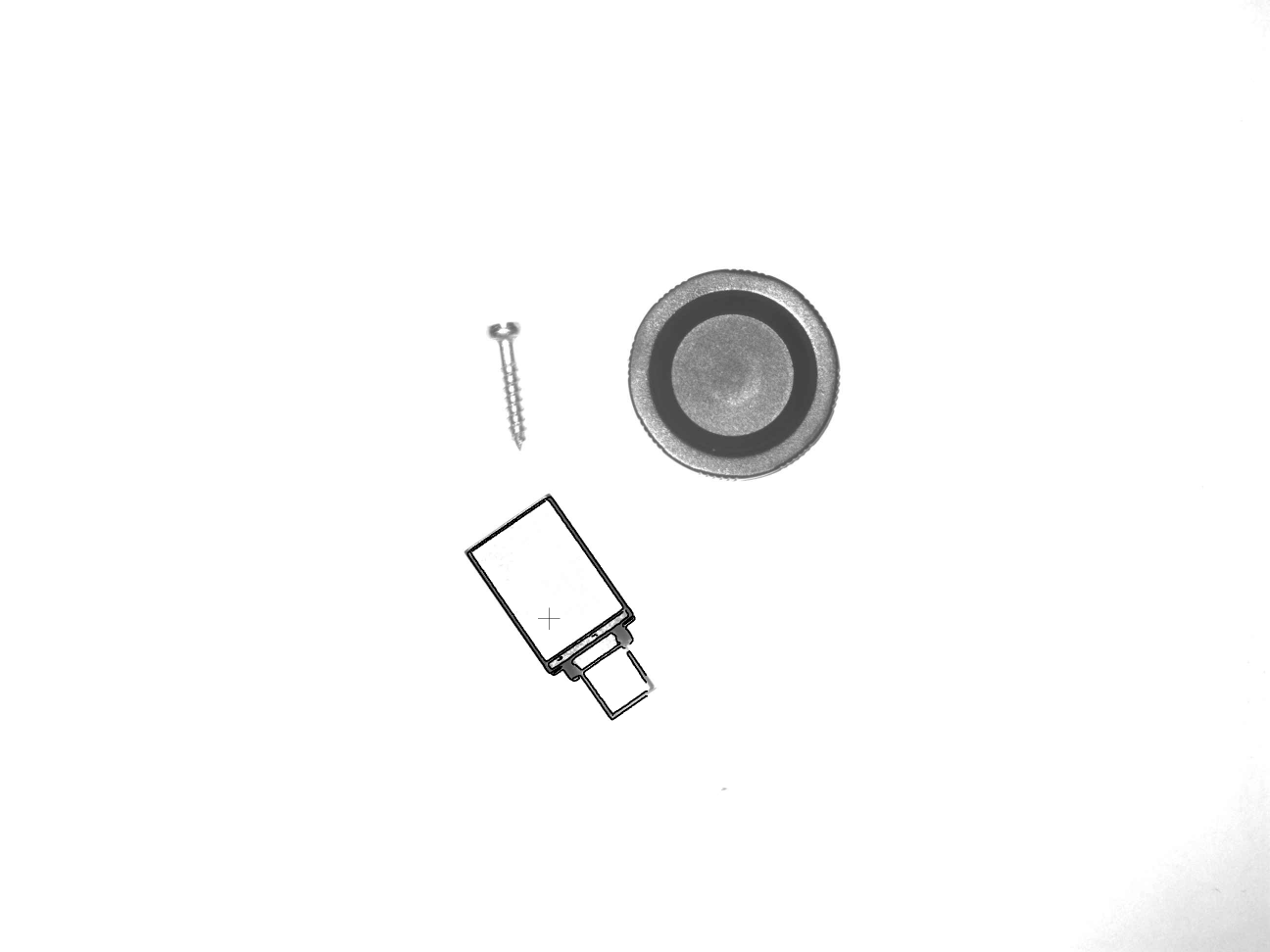
The scale samples are designed for exactly this: the same set of parts photographed at three working distances, the parts shrinking from near to far. Take the square connector (a rectangular body with a protruding tab below, dark contour, non-rotationally-symmetric) from the nearest image (sample 1) as the model, and search all three images over a scale range of \([0.55, 1.20]\) (step 0.05):
| Scale sample | Solved scale | Solved angle | Score |
|---|---|---|---|
| 1 (nearest, template source) | 1.000 | \(0^\circ\) | 97.8 |
| 2 (middle) | 0.850 | \(-2^\circ\) | 88.0 |
| 3 (farthest) | 0.650 | \(-2^\circ\) | 74.4 |
The three images solve at scales 1.000, 0.850, and 0.650 — the part shrinks to 85% and then 65% of its original size as the camera pulls back, and the scale search recovers every step (Figure 17.4). The score falls with scale (97.8→88.0→74.4) because a smaller part has fewer effective edge points and the soft edges of a real photograph become harder to work with, but 74.4 is still far above minScore=25 and the localization is solid. The redrawn model contour, scaled by the solved factor, wraps each differently sized connector snugly.
Scale matching fills in the fourth degree of freedom of the pose; it does not replace calibration (Chapter 5): when the working distance changes, the pixel-to-millimeter conversion changes too, and accurate dimensional measurement still requires recalibration. What scale matching solves is only “can we still find it after the working distance drifts, and by how much did it scale.”
17.5 Template Design
Not just any part in the samples can serve as a template, and this real dataset happens to lay three lessons out in the open.
First, the template must break rotational symmetry. Imagine modeling on that ring washer: a circle’s contour rotated by any angle is still the same circle, so the vast majority of edge points in the model are “direction-consistent” with every angle; the score stays high but the reported angle is pure chance — the classic rotational-symmetry trap. This chapter chose the pentagonal wedge precisely because its vertical edge and chamfered corner contribute a large number of edge points with unique directions, so the angle can be locked firmly (the angle residuals of all six instances are small). The lesson in one sentence: the score only guarantees “the contour lined up,” never “the pose is the unique solution” — checking whether a template is (approximately) rotationally symmetric should be a fixed step before modeling.
Second, features must be one of a kind. The toothed rack in the samples is a row of repeating square teeth; were it the model, any equally spaced square-wave edge in the scene could claim a high score as an impostor. The wedge’s combination of edge segments is unique among this set of parts, which is why every distractor is rejected. The template should be a one-of-a-kind combination of structures, and the threshold must sit above the highest score any distractor could earn.
Third, the edges of a real photograph are soft. The scale samples are real grayscale photos of metal parts, with edges only a few pixels wide and carrying reflections and noise. Box-average downsampling them directly drives the gradient magnitude below the contrast threshold, so that not even the part’s own image can be matched; matching must be done at full resolution, with the pyramid limited to 2 levels (automatic layering wipes out the soft edges at the upper levels and the coarse screen fails). The silhouette samples have extremely high contrast, so none of these concerns arises — which itself shows that the “edge quality” of the template and samples directly dictates how the parameters must be set.
17.6 SciVision Implementation
First, a naming trap: the SDK’s SciSvOCV is not contour matching — OCV is optical character verification, for character-defect verification. Contour matching and scaled contour matching are handled uniformly by SCIMV::SciSvScaleShapeMatch: scaleExtent=0 gives pure contour matching, a nonzero range gives scale matching — one class covering both uses. Training and search:
SCIMV::SciSvScaleShapeMatch sm;
SciROI mask; // must be UNDEF: a GenRect1 rectangle raises 120001037
SciMatchModel model;
sm.CreateScaleImageModel(tmplImg, mask, /*pyramidLevel*/ 2, // 2 levels for soft edges; -1 (auto) is fine for silhouettes
/*startAngle*/ -180, /*angleExtent*/ 360, /*angleStep*/ 1,
/*startScale*/ 1.0f, /*scaleExtent*/ 0.0f, /*scaleStep*/ 0.05f,
/*lowerContrast*/ -1, /*upperContrast*/ -1, // edge hysteresis thresholds, -1 = auto
/*filterCoefficient*/ 3.0f, /*filterLength*/ -1, // training-side smoothing
/*minContrast*/ -1, /*optimization*/ -1,
/*polarity*/ 0, /*preGeneration*/ 1, &model); // preGeneration must be 1
SciPointArray centers; SciVarArray angles, scales, scores;
sm.FindScaleImageModel(sceneImg, searchROI, model,
-180, 360, 1.0f, 0.0f,
/*minScore*/ 40, /*matchCount*/ 3, /*overlapRatio*/ 40,
/*subpixel*/ 0, /*endLevel*/ 0, /*clutter*/ 0.0f,
/*coarseScore*/ 35, /*partialThreshold*/ 0.5f, /*spreadWinSize*/ 2,
¢ers, &angles, &scales, &scores);On the training side, the two triplets of angle and scale parameters mean the same; lowerContrast/upperContrast are the hysteresis double thresholds of the template’s edge extraction, deciding which points enter the model list; polarity is the polarity switch of Section 17.1. On the search side, minScore/matchCount/overlapRatio control the threshold, the instance count, and deduplication; GetScaleTemplateContours retrieves the model’s edge contours — this chapter’s overlay figures are drawn exactly that way, redrawing them at the solved poses.
Pitfalls hit in our measurements, recorded faithfully. First, mask must be passed as a default-constructed UNDEF ROI: passing a GenRect1 full-template rectangle raises error 120001037 outright — the same family temperament as feature matching and color matching. Second, preGeneration must be 1 (full model pre-generation), or subsequent matching is unusable. Third, subpixel can only be 0: setting it to 1 (interpolated refinement) crashes outright with 0xC0000005; setting it to 2 (least-squares refinement) “drifts at high score” — a high score carrying an angle error of tens of degrees, all the more deceptive. Fourth, soft-edged real photos require limiting the pyramid levels and matching at full resolution: if this chapter’s scale samples are box-average downsampled as usual and searched with automatic layering (pyramidLevel=-1), not even the connector’s own image can be matched (“match failure,” 122411002); switching to full resolution and pyramidLevel=2, all three images solve their scales cleanly. Note also that coarseScore must be \(\le\) minScore, or the coarse levels screen out qualified candidates. The complete project is at code/shape_matching/.
Industry Case: Switching Locators for Oily Workpieces
A machining shop needed pick-up localization on workpieces smeared with cutting-fluid oil and started with gray-value matching: the oil film made surface gray values undulate with the lighting angle, scores swung by as much as 30 points within a single day, and the threshold could not be tuned. Switching to shape matching stabilized things immediately — what the oil changes is the gray-value distribution, while the workpiece’s contour does not budge, and gradient-direction similarity is naturally immune. But the first version simply boxed the entire workpiece, sweeping all of the internal machining texture into the edge-point list: modeling and matching were both slow, and scores jittered whenever the oil locally wiped out some texture. The second version kept only the outer contour and two key locating holes, and both speed and stability passed. Two lessons: shape matching’s robustness comes from “comparing only the reliable edges,” and stuffing unreliable detail into the model is self-sabotage; template design matters as much as algorithm selection.
17.7 Summary
- Shape matching abstracts the template into a list of edge points + gradient directions; the score \(s=\frac1n\sum\cos\Delta\theta_i\) is the average direction agreement: the model is a list of points with geometric coordinates, so it can search explicitly over angle and scale; gradient direction is unchanged by gain/offset and even by locally monotonic nonlinear mappings; missing points only dilute the score without disturbing the rest — searchability, illumination robustness, and occlusion tolerance all spring from the same source.
- Rotation robustness: a single pentagonal-wedge template finds all six instances across five real samples, with angles spanning \(-152^\circ\) to \(+102^\circ\) and scores all \(\ge 93.7\), and not one ring or toothed-rack distractor falsely detected; at the same rotated instance grayscale NCC is only 0.585 (\(< 0.80\)), confirming that NCC does not resist rotation.
- Under occlusion, score ≈ visible fraction: a synthetic bar covers 36% of the real wedge, the score goes 99.8→76.5 (degradation ratio 0.77), and the pose is still exact;
minScoreis the maximum tolerable occlusion fraction, and coarse-screening parameters such aspartialThresholdmust be opened up along with the occlusion budget. - Scale, the fourth dimension, is opened by
scaleExtent; as the real connector shrinks with working distance, the three images solve at scales 1.000 / 0.850 / 0.650 in turn. Scale matching completes the pose; it does not replace calibration. - On the SDK side, remember a few things: pass mask as UNDEF, preGeneration=1, subpixel only 0, coarseScore \(\le\) minScore; soft-edged real photos must be matched at full resolution with the pyramid limited to 2 levels, or not even the part’s own image can be matched.
Shape matching solves the hardest form of “where is the part”; when the target is not a rigid contour but a color blob or texture features, feature matching and color matching remain as options (Chapter 18). Edge-based shape matching has two further classic threads: Borgefors’s hierarchical chamfer matching measures contour similarity via a distance transform (Borgefors 1988), and Belongie et al.’s shape contexts describe point-set shape with distribution histograms and solve the correspondence (Belongie, Malik, and Puzicha 2002). The principles and engineering details of shape matching are treated most systematically in the book by Steger et al. (Steger, Ulrich, and Wiedemann 2018).