41 3D Measurement
After a point cloud has been registered and aligned (Chapter 39) and filtered clean (Chapter 37), what the production line actually wants is not a pretty cloud of points but numbers — what is this workpiece’s step height, is the circular land large enough, is the mating face flat, is there a local raised defect. Computing these numbers and deciding pass or fail on their basis is exactly what 3D measurement does. This chapter is the three-dimensional counterpart of the two-dimensional measurement methodology of Chapter 21: the measurement chain is still point cloud → fitted primitive → geometric quantity → judgment, and the role of each stage, how error propagates, and why band-width tolerances and dimensional tolerances differ statistically all map one-to-one onto the 2D case — only the primitives are promoted from lines and circles to planes, and the evaluation switches from pixels to millimeters.
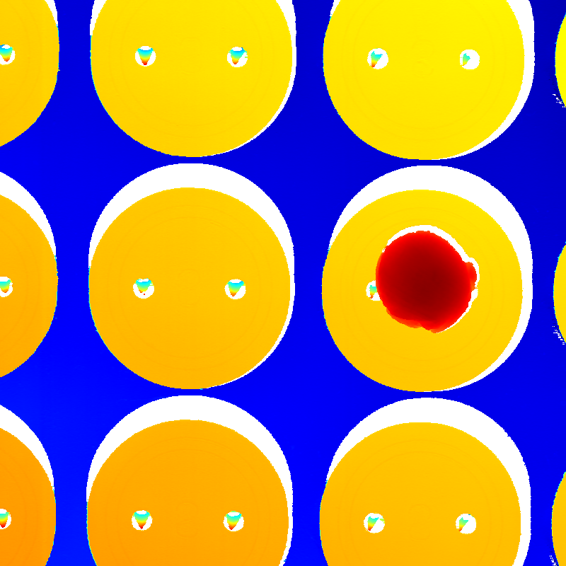
The experimental object (Figure 41.1) is a real Smart3 range image (sample/height01.srt, 1600×1600, taken from the SDK’s “height measurement” example scheme): a precision-machined part, about 19.2×19.2 mm in top view, with a lateral resolution of \(0.012\) mm/pixel and a vertical \(0.001\) mm/count. The surface structure is a sunken grid-channel floor, above which sits an array of raised circular boss lands, each carrying two small dimples, and one of which also has a pronounced local raised bump defect. This is real scan data: there are no analytic ground-truth labels, so every number is reported faithfully as a measured value; the roughly 260k unhit pixels (raw count 0) are the invalid background, skipped point by point.
41.1 Fitted Primitives: Planes and Circles
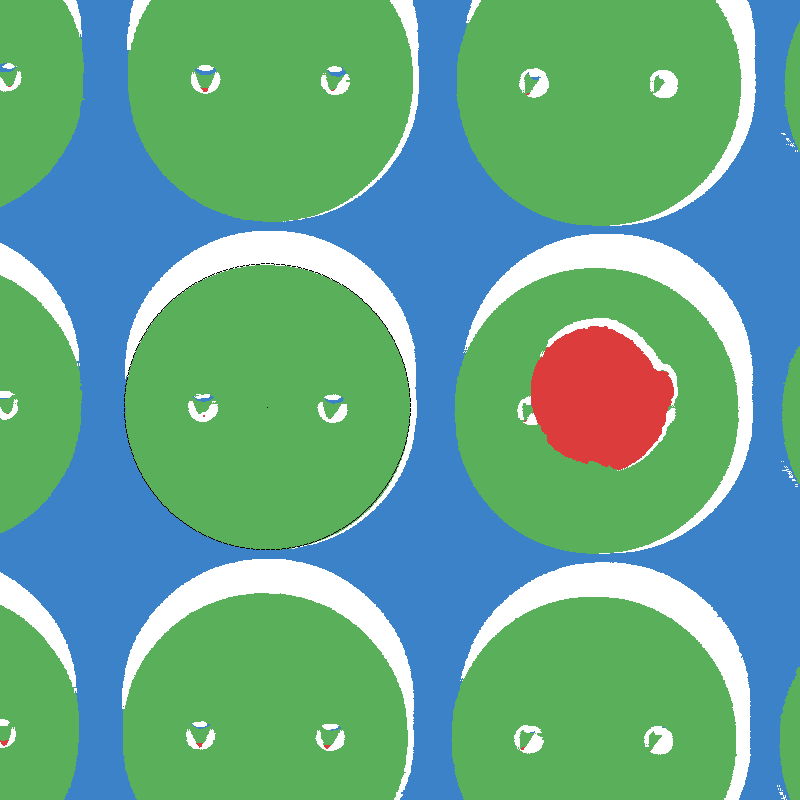
The primitives of 2D measurement are lines and circles (Chapter 14); the workhorse in 3D is the plane. Before fitting, the whole point cloud must first be segmented onto its individual feature faces (Figure 41.2). Here the step (≈4.4 mm) is far larger than the workpiece’s fixturing tilt on the stage (±0.6 mm), so a single global height threshold \(z=33.5\) mm cleanly bisects the channel floor (about 31.2 mm) from the lands (about 35.6 mm); a real production line accomplishes the same step via region growing, normal clustering, or nearest-face assignment to a registered CAD model. After splitting, the transition walls and flying points must be rejected: the side-wall pixels between land and channel straddle the dividing threshold, so we fit once, then discard points whose residual exceeds \(0.1\) mm and refit — what remains is a clean set of plane points.
Least-squares plane fit fits a face’s point cloud to \(z=ax+by+c\), with the three coefficients solved in one shot from a set of \(3\times3\) normal equations:
\[ \begin{bmatrix}\sum x^2 & \sum xy & \sum x\\ \sum xy & \sum y^2 & \sum y\\ \sum x & \sum y & N\end{bmatrix} \begin{bmatrix}a\\b\\c\end{bmatrix}= \begin{bmatrix}\sum xz\\ \sum yz\\ \sum z\end{bmatrix}. \]
This is precisely the three-dimensional landing of the “least-squares solution of an overdetermined system” from Chapter 2, with the unknowns going from two (a 2D line) to three. Once the coefficients are solved, the plane’s unit normal is \(\mathbf n=(-a,-b,1)/\sqrt{a^2+b^2+1}\) and the intercept is fixed by the centroid. The fitted channel floor is \(z=-0.0151x+0.0250y+31.217\), with its normal tilted 1.675° from vertical — this is the workpiece’s actual fixturing tilt on the stage; in real data it is always present, and when measuring the step and parallelism below we must work along the datum-face normal rather than along the \(z\) axis, so as not to bake this tilt into the result.
The robustness of plane fitting shares the same origin as in 2D: a few outliers (flying points, side-wall pixels) pull the least-squares datum off, and industrial implementations commonly layer on an iterative reweighting (IRLS) or a RANSAC pre-screen. This chapter uses the most elementary “fit → reject by residual threshold → refit” in two rounds, already enough to squeeze the channel floor’s RMS down to 19.0 µm.
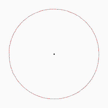
Circle fit and “what a range image can see”. The diameter of a circular land is measured with a Kasa circle fit: project the outline points of the land’s connected component onto the \(xy\) plane and solve a \(3\times3\) normal-equation system isomorphic to the plane fit, yielding the center and radius in one step. There is a key realization about real data here — a range image is a 2.5D height field that sees only upward-facing surfaces, not vertical side walls. So a land leaves only a circular outline in the range image (from which a diameter can be fitted), while its side wall as a cylinder segment is simply not sampled; fitting a true three-dimensional cylinder (axis + radius, five unknowns) requires multi-view scanning or a full point cloud, which a single top-down range image cannot provide. Here we take a non-edge, largest interior land, bin its boundary by angle and keep only the maximum-radius outline point in each direction (cleanly excluding the boundaries of the two inner dimples), and fit a diameter of 6.8608 mm (radius 3.4304 mm), with a roundness (radial peak-to-valley) of 86.4 µm (Figure 41.3).
41.2 Step, Parallelism, and Height Measurement
Once the primitives are in hand, the geometric quantities are closed-form formulas that themselves introduce no new error (the same as in Chapter 21).
Step (plane-to-plane distance) — exactly the core of this sample’s “height measurement”. The height difference of the land relative to the channel floor equals the signed perpendicular distance from the land’s centroid along the channel-floor normal to the floor. Measured at 4.3915 mm. Each face is fitted from nearly a million points, and the step fully inherits their sub-micron stability. It is worth stressing “along the normal” rather than “along the \(z\) axis”: the workpiece is fixtured with a 1.675° tilt, and taking the vertical height difference directly would differ by a factor of \(\cos\theta\) (about a 4 µm systematic bias), so engineering practice always takes the step as the perpendicular distance along the datum-face normal.
Face-to-face angle / parallelism. The angle between two planes is given by the dot product of their normals, \(\theta=\arccos\lvert\mathbf n_1\!\cdot\!\mathbf n_2\rvert\) — the 3D counterpart of the line-line angle of Chapter 21 (a normal is to a plane as a direction vector is to a line). The normal angle between the channel floor and the lands measures 0.1085°, close to 0, confirming that the upper and lower face groups of this machined part are indeed parallel — that is, the 1.675° overall tilt is a fixturing-induced rigid-body pose shared by both faces, which cancels out upon differencing and does not contaminate the step. This “common-mode tilt cancels automatically when differencing between faces” is the fundamental reason 3D measurement evaluates against a datum face rather than the world coordinate system.
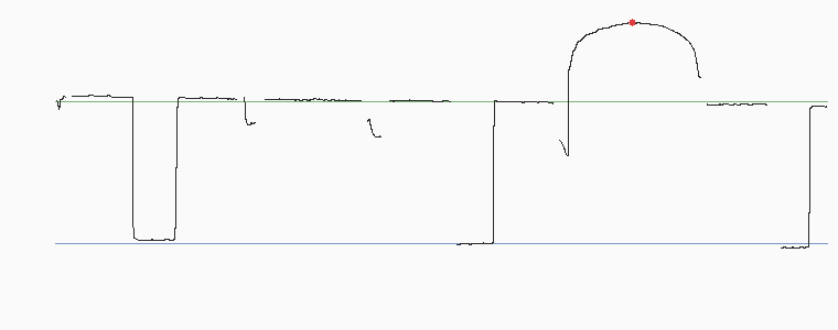
Plotting the \(x\)–\(z\) cross-section of the land array along the row through the bump peak (Figure 41.4), the step and the protrusion are immediately clear: the black polyline drops about 4.4 mm back and forth between the land level (green line) and the channel floor, and the dome bulging above the green line in the center is the bump defect.
Pulling the measured geometric quantities together (Table 41.1). Here two classes of quantity must be distinguished: averaging-class quantities like the step and the diameter become monotonically more stable as the point count grows, with the deviation settling at the \(\sigma/\sqrt N\) floor; whereas the band-width-class quantities of the next section — flatness, roundness — do exactly the opposite, with the expected range growing as more points are added, so the number is pushed up by the sampling density. The same point cloud, the same noise, yet the two classes respond to “point count” in completely opposite directions — this is the most easily misread point in a 3D measurement report, and is why band-width quantities must always be reported together with the sampling conditions.
| Geometric quantity | Measured | Note |
|---|---|---|
| Step / channel floor → land (mm) | 4.3915 | along datum normal, this sample’s main measurement |
| Parallelism floor ∠ land (°) | 0.1085 | ≈0, confirms the two faces parallel |
| Fixturing tilt (°) | 1.675 | floor normal vs vertical, rigid-body pose |
| Circular land diameter (mm) | 6.8608 | Kasa circle fit of the outline |
| Land roundness (radial P2V, µm) | 86.4 | RMS 12.0 |
| Channel floor flatness, least-squares P2V (µm) | 225.5 | RMS 19.0 |
| Channel floor flatness, minimum zone (µm) | 194.3 | ≤ least squares |
| Land-array flatness, least-squares P2V (µm) | 255.4 | RMS 22.3 |
| Land-array flatness, minimum zone (µm) | 234.2 | ≤ least squares |
| Bump defect above land (mm) | 2.5180 | lateral scale ≈3.44 mm |
41.3 Flatness, Roundness, and GD&T
Beyond dimensions, drawings also carry the frames of geometric dimensioning and tolerancing (GD&T), which speak not of “how much is measured” but of a tolerance zone: the toleranced face must lie entirely within a band of some thickness. This is fully consistent with the 2D tolerance-zone thinking of “parallelism/roundness/straightness” (Chapter 21), only the band is promoted from between two lines in 2D to between two faces in 3D. The zone for flatness is the thickness between two parallel planes, within which all points of the toleranced face must lie; the zone for roundness is the ring between two concentric circles. The starting point of this language is assembly function: as long as the toleranced face lies wholly within the zone, whatever its specific undulations, its mating with the counterpart is guaranteed. The universal recipe for evaluating them by vision is the same as in 2D: take the set of toleranced points, compute deviations against the evaluation datum, and max−min is the minimum band width needed to contain the point set.
Flatness. With the fitted plane as datum, the max−min of the points’ signed perpendicular distances is the peak-to-valley value (P2V). The channel floor measures 225.5 µm (least-squares evaluation, with an RMS of only 19.0 µm), and the land array 255.4 µm (RMS 22.3 µm) — the land-array number is slightly larger because it evaluates several mutually independent lands together, folding in the coplanarity error between lands rather than just the machining undulation of a single land. Figure 41.5 draws the residuals of the two faces as diverging heatmaps (±60 µm): the channel floor’s (left) long-range red-blue gradient is a large-scale plane waviness, while each land’s (right) concentric red-blue rings are a slight central doming — these are real topography left by machining and scanning together, not random noise. Note that flatness is an extreme-value statistic: the RMS is only a couple dozen microns, yet the P2V reaches a couple hundred, precisely because it is determined by the two most extreme points across the whole face, and the denser the sampling, the higher the chance of catching an extreme point and the larger the number.
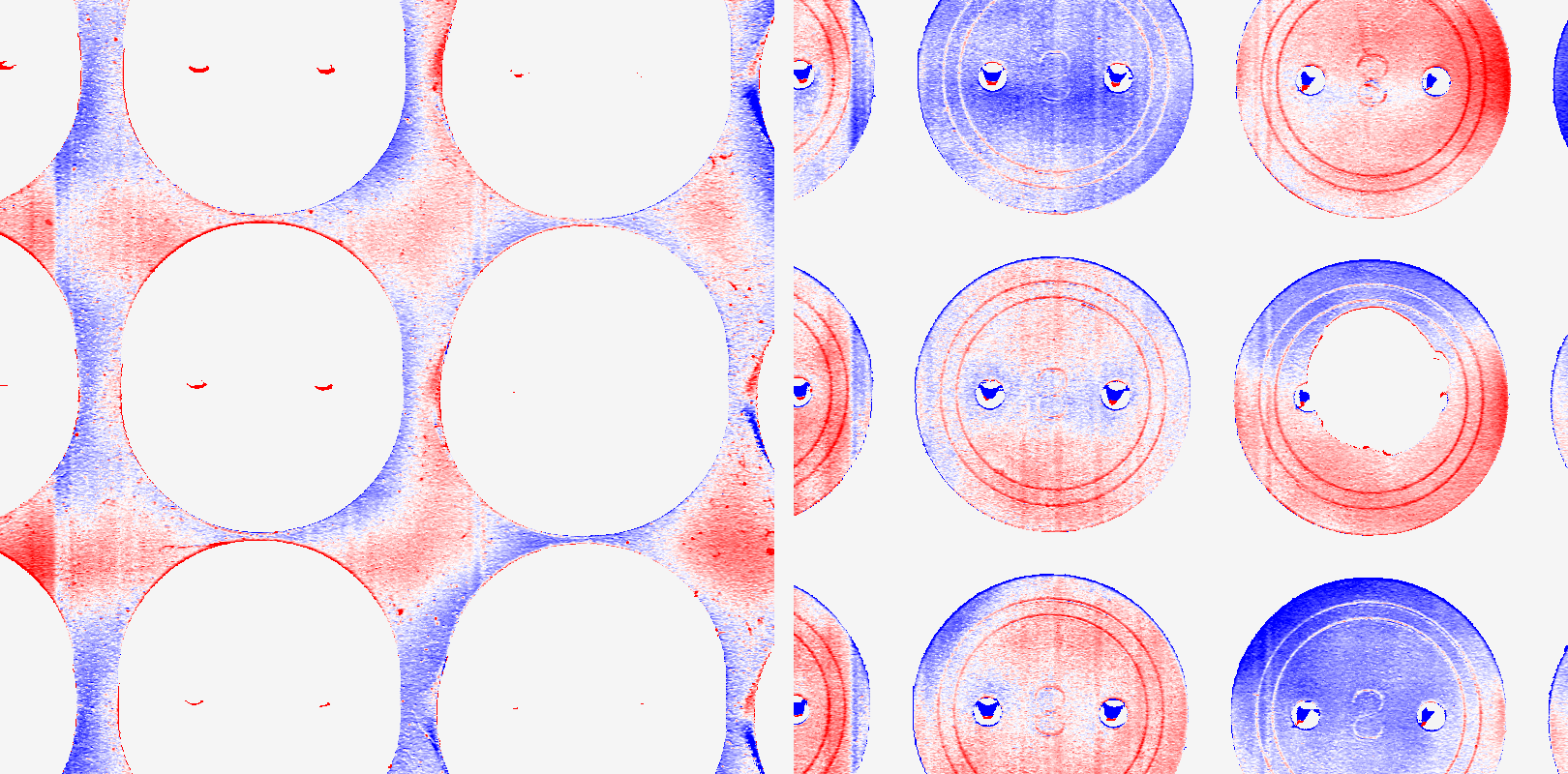
Roundness and the bump defect. The outline roundness of the land from the previous section is 86.4 µm (Figure 41.3) — the outline points hug the fitted circle evenly, with no systematic ellipse or polygon, showing the land’s outer edge really is a true circle. The bump defect, by contrast, uses a different criterion: its peak pixel rises 2.5180 mm above the land datum (lateral scale about 3.44 mm), located by connected-component segmentation and taking the perpendicular distance of the highest point in the component along the land normal. Such a local protrusion directly props up the mating face in assembly, and is a defect quantity that must be reported separately — a different language from a global band-width quantity like flatness.
Datum dependence. For the same set of points, switching the evaluation datum changes the flatness number: with the least-squares plane as datum the channel floor’s P2V is 225.5 µm, while with the minimum zone datum (fine-tuning the plane’s tilt to make the containing band thinnest) it is 194.3 µm; the land array correspondingly gives 255.4 µm and 234.2 µm. This is the 3D reprise of the 2D “datum dispute over roundness” of Chapter 21 — the minimum zone gives the thinnest band by definition and is the very embodiment of the GD&T semantics; least squares is the most robust but its band width is systematically larger. So any reported geometric tolerance must be reported together with its evaluation method, otherwise the numbers from two machines are not comparable.
Minimum zone ≤ least squares, always. The minimum-zone datum is chosen specifically, among all possible datum planes, as the one giving the thinnest containing band, and the least-squares plane is merely one particular solution among them, so the minimum-zone evaluation value is necessarily no larger than the least-squares evaluation value (in this chapter the channel floor 194.3 ≤ 225.5 and the land array 234.2 ≤ 255.4 — both pairs verify this inequality).
41.4 SciVision Implementation
The real range image is loaded with Sci3DFileOperation::LoadRangeImage (link Sci3DFileOperation.lib; rc=0 means success; it prints a harmless “Directory does not exist.” to stderr). GetValue(row,col) returns the raw count, which times ResolutionZ() gives the physical height (mm); a count of 0 is an invalid pixel. The geometric quantities are provided by SciSv3DGeometryMeasure, and the geometric tolerances by SciSv3DGDTTools. Compared with 2D there is one key difference that must be written down faithfully: the 3D GDTTools return deviation values in real mm units, rather than the normalized \([0,1]\) scores of the 2D SciSvGDTTools in the neighboring chapter Chapter 42 — this chapter’s ChebyshevFlatness returns 0.19731 and Parallelism returns 0.26143, both genuine millimeter deviations that can be thresholded directly against the drawing tolerance.
The per-API on-machine measured status (the 3D module is broadly crash-prone/silent, see the engineering conventions for details; every SDK call is fed the same robustly-rejected point set as the hand-written main chain):
- Working and matching the hand-written version:
LeastSquarePlaneFit(channel floor meanErr 0.01905 mm = 19.0 µm, agreeing to four digits with the hand-written RMS; land 0.02229 mm),AngleFromPlanes(0.10861°, agreeing to four digits with the hand-written parallelism 0.1085°),ChebyshevFlatness(minimum zone 0.19731 mm = 197.3 µm, differing from the hand-written minimum zone 194.3 µm by only 3 µm, forming a strong cross-validation),Parallelism(0.26143 mm = 261.4 µm, of the same magnitude as the hand-written land flatness 255.4 µm). - Failing:
PlanesDistancereturns error code 123501017 and yields 0 (a defect in its strict-parallelism tolerance check) — so the step is computed by hand instead (the perpendicular distance of the land centroid along the channel-floor normal, 4.3915 mm). - Inert, no output:
ResidualFlatnessreturns 0, unusable.
On this machine the 3D module is broadly crash-prone or silently returns 0, so SDK calls are uniformly placed in a subprocess probe: after the main process has produced its figures and numbers, it re-invokes its own sdkprobe branch via system() to poke the SDK, and a crash merely exits the subprocess without dragging down the main chain. This phase separation of “hand-written main chain, SDK as corroboration” is the uniform engineering strategy across the 3D chapters of Part IX of this book.
SciRangeImage ri;  SCIMV::Sci3DFileOperation fop;
SciVar path("sample\\height01.srt");
long rc = fop.LoadRangeImage(path, &ri, false);          // rc=0 means success
double z_mm = ri.GetValue(row, col) * ri.ResolutionZ();  // raw count -> physical height mm (0 = invalid)

SCIMV::SciSv3DGeometryMeasure gm;
Sci3DPlane floorPlane, bossPlane;  double meF = 0;
rc = gm.LeastSquarePlaneFit(floorA, 5.0, 5.0, 1, &floorPlane, &meF);  // meanErr 0.01905 mm
double ang = 0;                                          // parallelism: arccos of normal dot product
rc = gm.AngleFromPlanes(floorPlane, bossPlane, &ang);    // 0.10861° (≈ hand-written 0.1085)

SCIMV::SciSv3DGDTTools gdt;
double fCheb = 0, par = 0;
rc = gdt.ChebyshevFlatness(floorA, 1, 0.0, &fCheb);      // minimum zone 0.19731 mm ≈ hand-written 0.1943
rc = gdt.Parallelism(bossA, floorPlane, 0, 0.0, &par);   // 0.26143 mm (real mm units)
// step: PlanesDistance fails (123501017) -> hand-written land-centroid perpendicular = 4.3915 mm
The engineering strategy is consistent with 2D: the entire measurement main chain uses hand-written least squares (plane/circle fitting are deterministic, reproducible “mathematical objects”), and the SDK is placed in a subprocess probe for corroboration. This brings two benefits: first, the hand-written implementation is deterministic and reproducible, unaffected by 3D-module crashes, so the main chain can always produce numbers; second, the usable SDK APIs serve as an independent second implementation for cross-validation — ChebyshevFlatness independently reproduces the minimum-zone flatness through a completely different code path (197.3 µm vs 194.3 µm), and LeastSquarePlaneFit’s meanErr aligns exactly with the hand-written RMS at 19.0 µm, and this “two implementations agreeing independently” is far more trustworthy than the self-corroboration of a single implementation. The complete project (including the generation of the five figures and all the prints of the subprocess probe) is in code/3d_measurement/.
Industry Case: Flatness Acceptance of Mating Faces
A machined mating face required flatness at the few-dozen-µm level, yet acceptance was repeatedly mired in disputes. The supplier first accepted with a coordinate measuring machine (CMM) probing points: sparse sampling (a few dozen points) missed the local warp at the mating-face edge, so the reported flatness was optimistically biased and judged passing. The customer switched to a 3D surface scan with full-coverage sampling; the warp was caught, but among the hundreds of thousands of points the scanner’s noise floor and fixturing tilt crept in too, and the flatness was pushed up by the extreme-value statistic — just as in this chapter’s real sample, where the channel floor’s RMS is only 19 µm yet the P2V reaches 225 µm, and the whole face carries a 1.675° fixturing tilt that, if not evaluated along the datum-face normal, adds yet another systematic bias. More thorny still was the evaluation method: the customer used the minimum-zone method (194 µm), the supplier the least-squares method (225 µm), and the same face yielded two numbers. The eventual resolution lay not in the algorithm but in the protocol — the inspection protocol stated three things in black and white: the evaluation method (minimum zone vs least squares), the sampling density (upper limit on point spacing), and the filter cutoff frequency. The lesson takes one sentence: a 3D measurement report must carry the triplet — the value, the evaluation method, and the sampling/filtering conditions; miss one, and the number has no comparability.
41.5 Summary
- The measurement chain is isomorphic to 2D: point cloud → fitted primitive (plane/circle) → geometric quantity (step/angle/diameter) → judgment (flatness/roundness/defect); the geometric-quantity stage is exact formulas that introduce no new error, and the accuracy is entirely propagated from single-point noise through \(1/\sqrt N\) fitting. This chapter uses a real Smart3 range image with no ground-truth labels, so everything is reported faithfully as measured values.
- A range image is 2.5D and sees only upward-facing surfaces: a circular land leaves only a top-view outline (from which a diameter of 6.8608 mm can be fitted), while its cylindrical side wall is simply not sampled — a true 3D cylinder fit needs multi-view or a full point cloud, which a single top-down range image cannot provide.
- Common-mode tilt cancels when differencing between faces: the workpiece’s 1.675° fixturing tilt is shared by the upper and lower faces, and taking the step as the perpendicular distance along the floor normal (4.3915 mm) and the parallelism at 0.1085° both cancel it cleanly — this is the fundamental reason 3D measurement evaluates against a datum face rather than the world frame.
- Band-width quantities are extreme-value statistics: flatness (channel floor 225.5 µm / land 255.4 µm, both with RMS of only a couple dozen µm) and roundness 86.4 µm are all sensitive to sampling density, the opposite of “more accurate with more points” dimensional quantities.
- Datum dependence must be reported together with the evaluation method: for the same face, least squares gives 225.5 µm vs the minimum zone 194.3 µm (minimum zone ≤ least squares, always), and the SDK’s
ChebyshevFlatnessreproduces the minimum-zone value through an independent code path (197.3 µm) — reporting a geometric tolerance without the evaluation method is as good as not reporting it. - 3D SDK units differ from 2D: the 3D GDTTools return real mm values (not the 2D normalized \([0,1]\) scores); the usable APIs agree with the hand-written version (plane-fit meanErr 19.0 µm, angle 0.10861°, minimum-zone flatness 197.3 µm), but
PlanesDistancefails andResidualFlatnessis inert, so the main chain still relies on hand-written least squares with the SDK as corroboration.
For a systematic treatment of uncertainty analysis for 3D geometric quantities and minimum-zone evaluation, see further the book by Steger et al. (Steger, Ulrich, and Wiedemann 2018). The geometric tolerances used in this chapter have their symbolic language and tolerance-zone definitions fixed by geometric dimensioning and tolerancing (GD&T) standards: the international system is ISO 1101 (International Organization for Standardization 2017); for the flatness of a single face, ISO 12781 further specifies the vocabulary and parameters (including the minimum-zone and least-squares reference-plane definitions) (International Organization for Standardization 2011b), with the counterpart for cylindricity given in ISO 12180 (International Organization for Standardization 2011a). The “least squares vs minimum zone” datum dispute touched on repeatedly in this chapter is treated specifically in the form-error fitting literature, where Moroni and Petrò compare the principles and costs of various minimum-zone fitting algorithms (Moroni and Petrò 2008).