27 1D and 2D Barcode Recognition
Up to this point, every algorithm in this book has answered questions like “where is the target,” “what are its dimensions,” “is there a defect.” The recognition part of the book, which begins with this chapter, answers a different question: what is written in the image — turning pixels back into data. The most mature, largest-scale “image to data” application on the factory floor is the barcode: every workpiece, every circuit board, every box of material carries a printed or marked code, every station on the line reads it once, and the entire supply chain’s traceability system is built on those reads. Reading codes sounds easy — everyone scans codes with a phone — but codes on a production line are battered in turn by ink spread, lens defocus, low resolution, and smudging, and a single misread causes a part-mixing incident far more expensive than a failure to read. This chapter uses one real multi-symbology 1D barcode test card (Figure 27.1) to thread together four sets of experiments — 1D decoding, robustness boundaries under degradation, 2D error-correction comparison, and print-quality grading — and closes with a “hand-written encoder + SDK decoder” round-trip experiment.
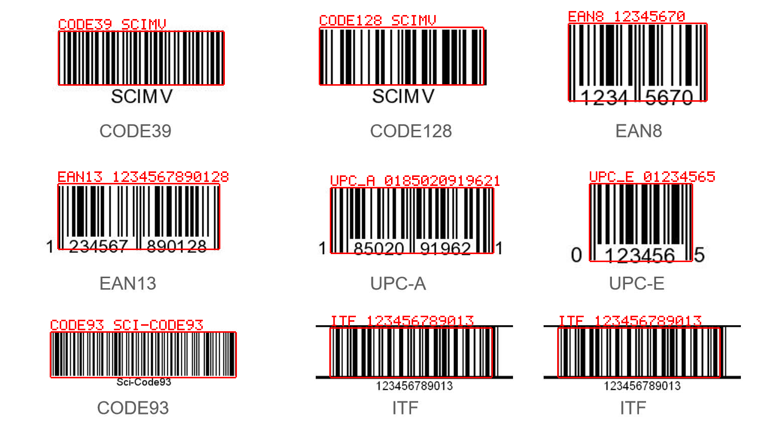
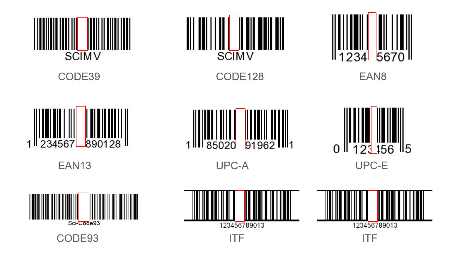
sample/barcodes.jpg (1536×878 grayscale): a standard card carrying 8 symbologies / 9 symbols — top row: CODE39 and CODE128 both encoding “SCIMV”, EAN-8 encoding 12345670; middle row: EAN-13 encoding 1234567890128, UPC-A encoding 185020919621, UPC-E encoding 01234565; bottom row: CODE93 encoding “Sci-Code93”, two ITF (Interleaved 2 of 5) both encoding 123456789013. The red boxes and red labels are SciVision FindBarcode detections overlaid (symbology name + decoded string).
27.1 1D Barcode Principles
The encoding idea behind a 1D barcode is remarkably plain: carry the data in a sequence of bar and space widths. The narrowest bar/space width is called the module; every other element’s width is an integer multiple of it. A character consists of a fixed number of bars and spaces, and the wide/narrow combination is that character’s code. The information unfolds along one direction only — every row in the vertical direction carries the same content. This is both the reason a single scan line suffices for decoding and the root of its robustness weakness; Section 27.2 will make that point painfully concrete.
The common symbologies divide the work among themselves: CODE39 encodes one character with 9 elements (5 bars and 4 spaces, 3 of them wide), supports digits and uppercase letters, has a simple structure and variable length, and is extremely common on industrial labels — but beware that its check character is optional; the standard does not mandate it. CODE128 is denser, supports the full ASCII set, and mandates a check character. EAN-13/EAN-8/UPC are retail product codes: a fixed number of digits with the last as a check digit. CODE93 is a higher-density refinement of CODE39. ITF (Interleaved 2 of 5) is a digits-only continuous symbology — both bars and spaces carry information with no inter-character gaps, giving high density but, again, an optional check digit. The test card in Figure 27.1 places all 8 of these symbologies side by side, which is exactly what we need to compare how their constitutions differ under degradation.
Each CODE39 and ITF element has some “self-checking” property — a single wide/narrow misjudgment usually lands on an invalid codeword and is discarded; but the string as a whole has no mandatory check character, so character-level truncation or substitution goes undetected. ITF is also continuous and the densest of the lot, and this hazard will be confirmed by its repeated misreads in Section 27.2.
Scan-line decoding proceeds in four steps. First, locate the code in the image — a barcode region has strong single-direction texture with highly consistent gradient orientations, which allows fast localization of candidate regions and estimation of their orientation. Then lay one or more scan lines along the barcode direction and extract a gray-level profile. Run edge detection on the profile to convert the alternating bars and spaces into a width sequence. Finally, look the width sequence up in the symbology’s codeword table to recover the characters, and verify the start/stop characters (* for CODE39) and the check character (if present).
Running the SDK’s FindBarcode on Figure 27.1 (full project in code/barcodes/; since barcodeType has no “automatic” setting, the example tries each of the 8 candidate symbologies in turn and merges the results), all 9 symbols on the clean image decode on the first attempt, all oriented near 0° (the card lies horizontal), with pixels-per-module between 2.1 and 4.1 px/module — CODE93 the narrowest (about 2.1), EAN-8 the widest (about 4.1). Turning on checkQuality yields ISO/IEC 15416 print-quality grades, and the spread is striking: EAN-8 and UPC-E score a perfect 4.0, CODE93 3.0 (limited by modulation), CODE39 and EAN-13 2.0, CODE128 and UPC-A 1.0 (all limited by decodability), while the two ITF symbols grade 0.0 (F) — decodability is zero, the measured widths are pressed right against the codeword decision boundaries with essentially no margin. Decodability reflects the distance of the width measurements from the decision boundary; modulation reflects local contrast at the narrow elements. On one and the same card the best-printed code (EAN-8) and the worst (ITF) differ by a full 4 grades — which is exactly the value of the grading system: it measures not “did it read this time” but “how far from unreadable.”
ISO/IEC 15416 grades 1D print quality from 4 (A) down to 0 (F): decode, contrast, modulation, defects, decodability, and other parameters are measured separately on multiple scan lines, each line is graded by its worst parameter, and the line grades are averaged. An overall grade ≥1.5 can usually be read reliably, but with little margin left.
The value of the grading system is this: it does not answer “did it read this time,” but “how far is this code from becoming unreadable.” A grade-1.0 code that reads today will stop reading after a lens change or a bit of dirt; requiring a label grade of ≥2.5 or 3.0 at line acceptance is a far more reliable standard than “it scanned successfully during the site trial.”
27.2 Robustness Boundaries
A successful decode is only the starting point; what engineering really cares about is where the boundary lies. We subject all 9 symbols of Figure 27.1 to four kinds of progressive degradation — Gaussian blur, additive noise, downsampling, and occlusion — recording the survival and misread status of each symbology at every level (Figure 27.2 shows four representative levels).
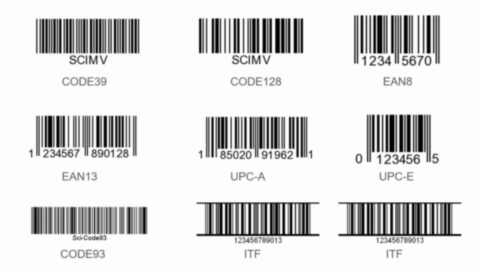
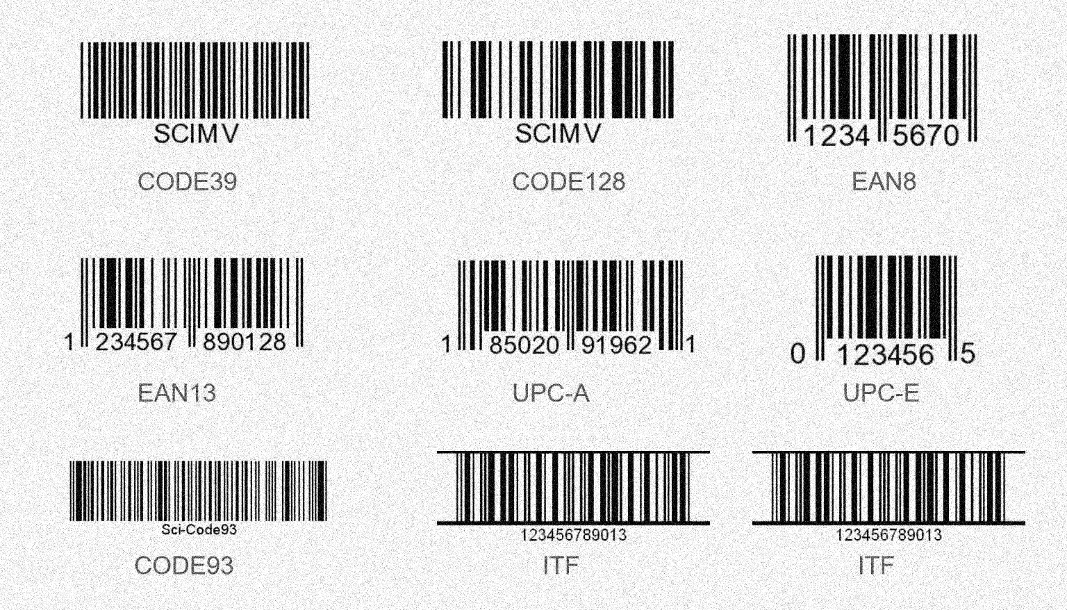
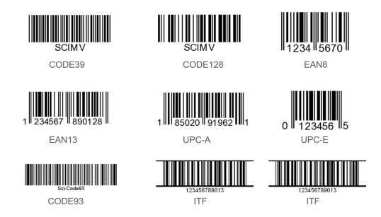
Each of the four boundaries carries its own meaning, and together they confirm the clean-image grade ordering item by item — the lower-graded codes fall first. Blur: all 9 codes are fine at \(\sigma=1\), 6/9 survive at \(\sigma=2\), and the first to fall are exactly the narrowest-module CODE93 (about 2.1 px) and the two ITF (about 3.0 px); all are gone at \(\sigma=3\) — blur flattens the contrast of narrow bars and spaces, the narrowest codes die first, exactly matching the 15416 prophecy that ITF/CODE93 were already at the bottom. Noise: \(\sigma=10\) is harmless, only UPC-A drops out at \(\sigma=30\), and 6/9 still survive at \(\sigma=50\) — multiple scan lines provide a natural averaging effect against random noise, with considerable margin. Resolution: 6/9 survive at ×0.5, and at ×0.35 only the 3 widest, steadiest codes remain (the two SCIMV and EAN-8, original ppm about 3.7–4.1, ≈1.3–1.4 px/module after scaling), with all gone at ×0.25 — 1D decoding only needs to resolve bar/space widths along a scan line, so its resolution requirement is far more lenient than intuition suggests, about 1.5 px/module being the practical floor here, and the narrowest CODE93 dies first the moment we downsample (for lens and resolution selection see Chapter 3).
The line most worth reading character by character is not which code fails to read, but which one reads wrong. At blur \(\sigma=2\) one ITF does not report failure — it decodes as 120000000013 (true value 123456789013); at 2% and 5% occlusion the other ITF is misread as 123400789013; and at scaling ×0.5 a nonexistent EAN-8 even appears, misread as 45252921. For a traceability system this is far more dangerous than a no-read: a no-read triggers a manual rescan, but a misread that goes unnoticed lets one workpiece travel the entire line wearing someone else’s identity. The root cause is the foreshadowing planted earlier — the check digit of ITF (and CODE39) is optional and absent on this card; ITF is also a continuous symbology (both bars and spaces encode, with no inter-character gaps), so local damage easily collapses a segment into another valid even-length digit string that the symbology layer cannot notice, which is also why it grades F for decodability even on the clean image. There are two engineering countermeasures: either choose a symbology with a mandatory check character (CODE128 never once misreads in this experiment), or enable the optional check digit for ITF/CODE39 and turn on codeCheck verification at the decoder; beyond that, validating the content format (digit count, prefix) at the application layer is always worthwhile.
Occlusion best separates the codes by constitution: a white stripe running the full height of the barcode, widened step by step as a percentage of each code’s width — at 2%, 6 of the 9 still read (the more forgiving CODE39/CODE128/EAN family survive, while the densest CODE93 and ITF have already fallen); at 5% only the two SCIMV remain; at 10% all fail. But “can be read” does not equal “is read correctly”: the two ITF misreads above occur exactly at the 2% and 5% occlusion levels. The reason is structural: a 1D barcode’s redundancy exists only in the vertical direction — the same content is repeated over the entire bar height, and any single horizontal scan line can decode it, so smudges from above or below are not fatal; but horizontally each character is encoded exactly once, with no error correction at all, and a full-height vertical occlusion that wipes out one character wipes out its only copy. To survive horizontal damage, the redundancy must be encoded into the data itself — which is precisely the design starting point of 2D codes.
27.3 2D Codes and Error Correction
DataMatrix (ECC200) is the most common 2D code on industrial parts. Figure 27.3 (a) is a 16×16 symbol: the entire left column and bottom row form the solid L-shaped finder pattern, providing the position and orientation reference; the top row and right column form the alternating black-and-white clock track, calibrating the row/column coordinates of the module grid; the remaining 14×14 data region places the codewords in the zigzag order prescribed by ISO/IEC 16022, with each codeword’s 8 bits arranged as a “Utah-shaped” module group.
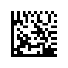
The robustness core of 2D codes is Reed-Solomon error correction. Intuitively it can be understood like this: treat the 12 data codewords as the coefficients of a polynomial and compute 12 additional check codewords over GF(256) to append after them — the 24 codewords are thereby bound by strong algebraic constraints, and when a few codewords are destroyed, the decoder can work backwards from the constraints to determine “which ones are wrong, and what their original values were.” The 12 check codewords can correct about 6 erroneous codewords at unknown positions — in this example only half of the 24 codewords are data: half the symbol area is spent on redundancy.
The Reed-Solomon error-correction budget: \(n_{\text{ecc}}\) check codewords can correct \(t\) erroneous codewords at unknown positions, subject to \(2t \le n_{\text{ecc}}\). Here \(n_{\text{ecc}}=12\), so \(t \le 6\): with 6 of the 24 codewords destroyed (25%), full recovery is still possible.
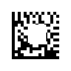
The occlusion experiment puts this “area for robustness” trade on the table: covering the symbol area with a white patch (placed off-center, avoiding the finder pattern), decoding is still correct at 10% and fails at 15% (Figure 27.3 (b)). Compared with the 1D codes — the most fragile ITF/CODE93 already fall at 2% full-height occlusion and all 1D codes are gone by 10%, with misreads before they die — the 2D code not only tolerates more, but crucially does not silently read wrong: when the error-correction budget is exceeded, ReadDM simply returns failure (rc=122703001) rather than a wrong value. Moreover, DataMatrix decodes correctly under blur \(\sigma=1,2,3\) and noise \(\sigma=30\) — levels at which half the 1D codes had already been wiped out (to be fair, the DM here is about 10.3 px/module, enjoying a resolution advantage over the card’s 2–4 px/module 1D codes, but the occlusion comparison is unaffected by this). It must be stressed that error correction is not free: for the same amount of data, a symbol with 50% redundancy needs twice the area; what the 2D code buys with area is the ability to survive horizontal damage — something a 1D code cannot buy at any area.
A word on the QR code: it belongs to the same “matrix code + Reed-Solomon” family as DataMatrix, the main difference being the localization scheme — QR uses three nested-square finder patterns at the corners, while DataMatrix uses the solid L-shaped edges; the former favors fast localization of large symbols at a distance, the latter is more compact for small-size direct part marking (DPM). The SDK provides a ReadQR interface, but this chapter’s test image contains no QR symbol, so no QR experiments were run; the principled conclusions carry over by analogy.
27.4 Round-Trip Verification Methodology
Where did the previous section’s DataMatrix image come from? There is a methodological question here worth unfolding: the SciVision SDK has only decoding APIs and no generation API whatsoever, and the testImage directory contains no 2D code images. To run the 2D experiments, we hand-wrote an ECC200 encoder (about 150 lines) in the example project: implement Reed-Solomon encoding over GF(256) (primitive polynomial 301; generator polynomial roots \(\alpha^1\!\dots\!\alpha^{12}\)), encode the text in ASCII mode (digit pairs compressed into one codeword, 253-state algorithm padding), then place the 12+12 codewords into the 16×16 symbol using the standard placement algorithm of ISO/IEC 16022 Annex F, and render the image with the finder pattern and clock track added.
The way to verify it is the round trip: hand the encoder’s image to the SDK’s ReadDM for decoding and compare the returned string character by character against the original “MVBOOK CH27”. Experimental result: decoding succeeds and the content matches; the symbol is 16×16 at about 10.3 px/module, with an ISO/IEC 15415 overall grade of 4.0 — a perfect score, exactly what an ideally rendered symbol should get. This round trip tests both ends at once: if the encoder places even one bit in the wrong position, decoding fails or the error-correction margin drops; and the SDK decoder reading back a perfect grade also proves that its grid localization and quality measurement work correctly. This is a reprise of the “gold-standard experiment” idea from Chapter 5 — test the entire chain with an input of known ground truth — and here the ground truth was encoded by our own hands, every bit traceable. It also demonstrates another use of the 15415/15416 grades: with a perfect-grade symbol as the baseline, a field symbol’s grade shortfall can be attributed parameter by parameter to the printing and imaging stages (for contrast problems caused by illumination, see Chapter 4).
27.5 SciVision Implementation
1D decoding is done by SCIMV::SciSvBarCode::FindBarcode:
SCIMV::SciSvBarCode bc;
Sci1DCodeArray codes; SciROIArray rects, bad;   // pass concrete objects for all three outputs
long rc = bc.FindBarcode(img, roi, SCI_CODETYPE_CODE39,
                         1,      // polarity: dark bars on light background
                         0,      // sampleRate: automatic sampling density
                         2,      // contrastLevel: medium contrast
                         4,      // codeNumber: expected count (headroom for per-symbology scan)
                         10000,  // timeOut: timeout (ms)
                         0,      // codeCheck: check-character verification switch
                         0,      // decodeDirection: decode in both directions
                         false,  // sendStartEnd: do not output start/stop characters
                         true,   // checkQuality: output ISO 15416 grades
                         &codes, &rects, &bad);
// Sci1DCode: codeType / codeString / orientation
//            / pixelPerModule / qualityLevel_15416
Three parameters deserve special mention. With codeCheck on, the check character is verified per the symbology’s rules — for CODE39 this requires the printing side to include the optional modulo-43 check character, but it is the symbology-level defense against the misread incident of Section 27.2. With checkQuality on, the per-parameter 15416 grades are output for each code — keep it on during line debugging and acceptance, and turn it off in stable production to save time. timeOut is the decoding timeout — stations with tight cycle times must set it, or a single poor-quality image can drag down the whole cycle.
DataMatrix decoding uses SCIMV::SciSvMatrixCode::ReadDM:
SCIMV::SciSvMatrixCode mc;
SciDMCodeArray ret; SciVarArray strs; SciROIArray cand;
long rc = mc.ReadDM(img, roi, 1 /*polarity: dark code on light background*/, -1 /*dmStyle: automatic*/,
                    6, 20,  // minSize/maxSize: search range for symbol rows/columns
                    30,     // minContrast: minimum contrast
                    0,      // mirror: detect mirroring automatically
                    1, 10000, 0,            // codeNum / timeOut / model
                    true,   // checkQuality: output ISO 15415 grades
                    false, false, false, false, false, false,
                    1, 1,   // decode and output strings both as UTF-8
                    &ret, &strs, &cand);
// SciDMCode: codeString / symbolRows / symbolCols
//            / moduleSize / orientation / qualityLevel_15415
Two engineering pitfalls. First, the symbology must be specified: FindBarcode’s barcodeType has no “automatic” setting, and asking for a symbology that is not in the image fails (returns a non-zero error code); when the symbology is unknown, the only option is to loop over a candidate list as this chapter’s example does (here it calls FindBarcode once for each of the 8 1D symbologies and merges/dedupes) — but a production project should pin the symbology down at the design stage, as part of the specification agreed with the label supplier. Second, header files such as SciSvBarCode.h unconditionally define their export macro as dllexport; placing their #include after the other dllimport-style headers makes linking work normally.
Industry Case: Read Rate from 98% to 99.9%
The DataMatrix read rate on an assembly line was stuck at 98% — which sounds high, but it means 20 manual rescans per thousand parts, unacceptable for both cycle time and labor cost. The project team first tweaked the decoding parameters repeatedly with little effect, then measured the labels with a verifier: modulation was only grade C — the label stock absorbed ink, causing ink spread and collapsing the contrast of the narrow elements; auditing the optical chain at the same time revealed a module width of only about 1.8 px/module, right at the decoding floor. Two corrective actions: switch to high-contrast laminated label stock, bringing the grade back to A/B; and increase the lens magnification to reach 3 px/module. The read rate rose to 99.9%, and the decoding parameters ended up at their defaults. The lesson: for read-rate problems, check the print-quality grade and the pixels per module first, then go tune algorithm parameters — when the grade is failing, tuning parameters is just gambling at the boundary.
27.6 Summary
- 1D barcodes encode in bar/space widths and decode along scan lines; they have a full bar height of redundancy vertically but no error correction at all horizontally: on this 8-symbology card the densest ITF/CODE93 already fall at 2% full-height occlusion and all 1D codes are gone by 10%; the resolution floor is about 1.5 px/module (only the 3 widest codes survive ×0.35). The survival order under degradation confirms the clean-image 15416 grade ordering item by item.
- A misread is more dangerous than a no-read: on this card ITF (optional check digit, continuous symbology) misreads several times under blur \(\sigma=2\) and 2%/5% occlusion (e.g. 120000000013, 123400789013) and grades F for decodability even on the clean image — choose a symbology with a mandatory check character (CODE128 never misreads here), turn on
codeCheck, and validate the format at the application layer: at least one of these three defenses must be in place. - 2D codes use Reed-Solomon error correction to trade area for robustness: the 16×16 DataMatrix’s 12 check codewords can correct about 6 erroneous codewords, decoding remains correct with 10% of the area occluded, and beyond budget it returns failure rather than a misread — a horizontal-damage tolerance far above the 1D codes.
- When the SDK only decodes and never encodes, the hand-written encoder + SDK decoder round trip both fills the experimental gap and constitutes a gold-standard verification of both ends (here the round trip scored a perfect ISO 15415 grade of 4.0).
- The ISO/IEC 15416/15415 print-quality grades answer “how far from unreadable”: accept on grades rather than on trial reads, and for read-rate problems check the grade and the pixels per module first.
For a more systematic treatment of barcode recognition and decoding algorithms in industrial vision, see the book by Steger et al. (Steger, Ulrich, and Wiedemann 2018). The print-quality grading systems cited repeatedly in this chapter come from two core standards: the per-parameter grading method for 1D codes is specified by ISO/IEC 15416 (International Organization for Standardization 2016), and the symbol-quality grading for 2D codes (including Data Matrix and QR) by ISO/IEC 15415 (International Organization for Standardization 2011). The encoding, error correction, and reference decode algorithm of each symbology have their own dedicated standards: the codeword placement and Reed-Solomon rules of Data Matrix (ECC200) are in ISO/IEC 16022 (International Organization for Standardization 2006), and QR Code in ISO/IEC 18004 (International Organization for Standardization 2015) — when agreeing on a specification with a label supplier or reproducing this chapter’s experiments, the original text of these standards should be the authority.