39 ICP Registration and 3D Rectification
Scan the same workpiece once from each of two viewpoints and you get two point clouds; to stitch them into a complete surface, you first have to align them. To compare a scanned physical object against its designed CAD model and judge whether assembly is correct, you first have to “place” the measured cloud into the model’s coordinate frame. Before a robot can grasp a part from a bin, it first has to know that part’s precise pose relative to the gripper — three seemingly unrelated tasks that share one and the same skeleton: rigidly transform one point cloud onto another so that the two coincide as closely as possible. This is three-dimensional registration, and ICP (iterative closest point) is the workhorse algorithm that carries registration on the industrial floor.
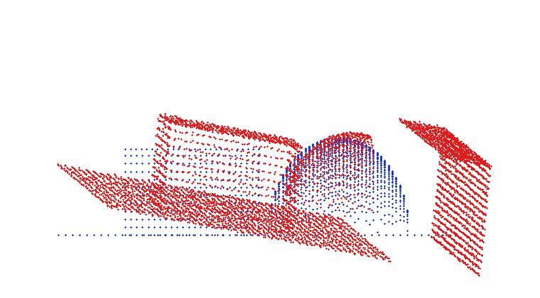
This chapter runs all of its experiments on a single synthetic scene (Figure 39.1): a model cloud (model) — a square box and a spherical cap sitting on a conveyor plane, 5678 points in all; and a scan cloud (scan) — obtained by applying a known rigid transform to the model (rotation of \(12°\) about the axis \((1,2,2)\), translation \((5,-3,2)\,\text{mm}\)), adding measurement noise with \(\sigma=0.1\,\text{mm}\), then cropping away one side and patching in, on the right, an “intruder wall” that does not exist in the model at all — 6497 points in all. Only 4310 points of the two clouds truly correspond; another 2187 points (33.7%) are non-overlapping with no correspondence. In the figure the model is blue and the scan is red, clearly misaligned at the start; that isolated red vertical wall on the right is the intruder structure — it has no corresponding point in the model, yet the algorithm must identify and exclude it. This “not fully overlapping” setup is not self-sabotage: in real scans, non-overlap from the camera’s field-of-view boundary, neighboring parts, and bin walls is almost the norm.
39.1 The Registration Problem and ICP
What rigid registration must solve for is a rotation matrix \(\mathbf R\) (\(3\times 3\), orthogonal with \(\det\mathbf R=1\)) and a translation vector \(\mathbf t\), such that transforming each point \(\mathbf p_i\) of the source cloud makes it coincide with the target cloud: \(\mathbf R\mathbf p_i+\mathbf t \approx \mathbf q_i\). This is the same problem as solving for the planar pose \((x,y,\theta)\) in 2D position correction in Chapter 19, upgraded to three dimensions — 2D has 3 degrees of freedom, a 3D rigid transform has 6 (3 rotational + 3 translational).
The difficulty is that we do not know which point of the source cloud corresponds to which point of the target cloud. The correspondence and the transform are each other’s cause and effect — knowing the correspondence lets you solve the transform, and knowing the transform lets you find the correspondence. ICP breaks this chicken-and-egg deadlock with a naive but effective iteration, doing three things each round:
- Find correspondences by nearest neighbor: transform the source cloud by the current estimate \((\mathbf R,\mathbf t)\), then for each source point find its nearest-neighbor correspondence in the target cloud. This step is ICP’s computational bottleneck and must use a kd-tree to reduce the brute-force \(O(NM)\) nearest-neighbor query to \(O(N\log M)\) (Chapter 37).
- Reject far correspondences: a nearest neighbor is not guaranteed to be a “true” correspondence — a point on the intruder wall also gets assigned a closest model point, but that correspondence is false. Rejecting outlier pairs by correspondence distance is ICP’s key gate for handling non-overlap. This chapter uses the median method: take the median \(\tilde d\) of all correspondence distances and keep correspondences with distance \(\le 2.5\,\tilde d\), shutting out large-distance correspondences such as the intruder wall.
- Solve for the optimal rigid transform: on the filtered correspondences, solve for the rigid transform that minimizes the sum of squared distances between corresponding point pairs. This step has a closed-form solution, namely the Kabsch / Umeyama algorithm.
The mathematics of the third step is worth unpacking; it is a beautiful application of the SVD from Chapter 2. Suppose after filtering there are \(n\) correspondence pairs \(\{(\mathbf p_i,\mathbf q_i)\}\), and we want to minimize
\[ E(\mathbf R,\mathbf t)=\sum_{i=1}^{n}\bigl\|\mathbf R\mathbf p_i+\mathbf t-\mathbf q_i\bigr\|^2 . \]
First subtract the centroid from each of the two point sets: \(\bar{\mathbf p}=\frac1n\sum_i\mathbf p_i\), \(\bar{\mathbf q}=\frac1n\sum_i\mathbf q_i\), and let \(\mathbf p_i'=\mathbf p_i-\bar{\mathbf p}\), \(\mathbf q_i'=\mathbf q_i-\bar{\mathbf q}\). One can prove that the optimal translation aligns the two centroids, while the rotation depends only on the centered points. Construct the \(3\times3\) cross-covariance matrix
\[ \mathbf H=\sum_{i=1}^{n}\mathbf p_i'\,\mathbf q_i'^{\,\top}, \]
take its singular value decomposition \(\mathbf H=\mathbf U\boldsymbol\Sigma\mathbf V^\top\), and then the optimal rotation and translation are
\[ \mathbf R=\mathbf V\,\mathrm{diag}(1,1,d)\,\mathbf U^\top,\quad d=\operatorname{sign}\!\bigl(\det(\mathbf V\mathbf U^\top)\bigr),\qquad \mathbf t=\bar{\mathbf q}-\mathbf R\,\bar{\mathbf p}. \]
That middle \(\mathrm{diag}(1,1,d)\) is the crucial stroke: a plain \(\mathbf V\mathbf U^\top\) may yield a “mirror” with determinant \(-1\) (a reflection rather than a rotation), and flipping the last column with \(d\) forces it back into the legitimate rotation group \(SO(3)\). Once \((\mathbf R,\mathbf t)\) is found, compose it onto the current estimate and proceed to the next iteration, until convergence.
Why centering + SVD? Expand \(E\), and after centering the translation term and the rotation term decouple: the optimal translation necessarily lands the transformed source centroid on the target centroid, and the remaining rotation term \(\sum_i\|\mathbf R\mathbf p_i'-\mathbf q_i'\|^2\) is equivalent to maximizing \(\operatorname{tr}(\mathbf R^\top\mathbf H)\), which under the orthogonality constraint is given optimally in one step by the SVD of \(\mathbf H\). This is precisely the direct realization of “SVD gives the optimal orthogonal approximation” from Chapter 2.
39.2 Convergence and Accuracy
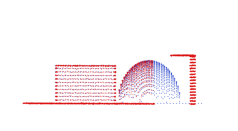
Give ICP a good initial value — here simply the identity matrix (at synthesis time the rotation is only \(12°\) and the translation a few millimeters, so the identity already lies within the convergence basin) — and run point-to-point ICP. The result: convergence in 58 iterations, final correspondence RMS 0.6443 mm, recovered rotation angle \(10.69°\) (GT is \(12°\), rotation-angle error \(1.97°\)), and translation error \(0.233\,\text{mm}\). Figure 39.2 shows the red scan cloud snugly hugging the blue model after alignment, while that intruder wall on the right still stands alone where it was — correspondence rejection correctly judged it non-overlapping and kept it from contaminating the transform estimate.
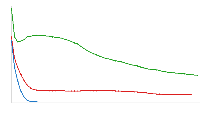
What is worth pondering is this \(0.6443\,\text{mm}\): it converged correctly (the pose is right) yet clearly stopped above the \(0.1\,\text{mm}\) noise floor. The reason hides in the cloud’s geometry — this cloud is dominated by a large expanse of conveyor plane, and the point-to-point metric has a congenital weakness on planes: a source point sliding along the tangential direction of the target surface barely changes its distance to the nearest target point, so the objective is nearly flat in the tangential direction. Each iteration can therefore move only a little, and convergence is slow and prone to stalling in a shallow minimum. The red curve in Figure 39.3 depicts this plainly: after the RMS drops quickly, it drags a long, nearly flat tail, crawling slowly toward the plateau over 58 iterations rather than crisply slamming into the noise floor.
Termination criterion: ICP usually stops when “the RMS change between two consecutive rounds falls below a threshold” or when “the maximum number of iterations is reached”. This chapter’s implementation stops when the RMS change is \(<10^{-5}\,\text{mm}\), with a 60-iteration cap as a backstop. Too loose a criterion quits early with insufficient accuracy; too tight a one spins idly near the noise floor — the long tail of point-to-point on a plane-dominated cloud is exactly the kind of scene where the criterion is hard to tune.
39.3 Local Minima: ICP’s Achilles Heel
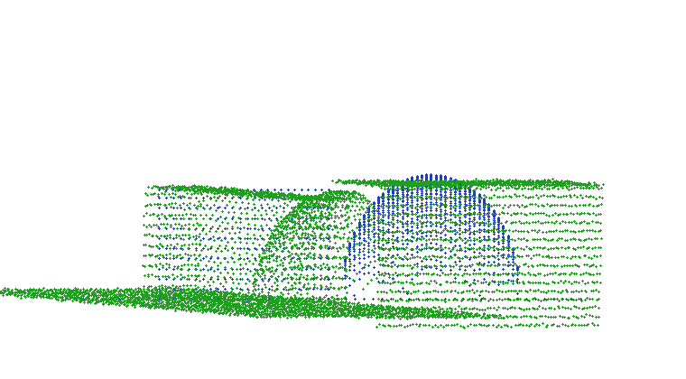
ICP only guarantees local convergence — it dutifully rolls down to the valley bottom nearest the initial value, but does not guarantee that this is the globally optimal valley bottom. To verify this, deliberately spoil the initial value: on top of the good initial value, add a further \(40°\) rotation about the \(Z\) axis, leave everything else unchanged, and rerun the same point-to-point ICP. The result is startling: the full 60 iterations are used up, with final RMS 2.0824 mm, rotation-angle error 29.3°, and translation error 8.20 mm. The green “aligned” result in Figure 39.4 is offset from the model as a whole — ICP converged, but converged to a wrong local minimum. The green curve in Figure 39.3 lingers high the whole way and never comes back down: the nearest-neighbor correspondences are mismatched from the start, the wrong correspondences solve a wrong transform, the wrong transform reinforces the wrong correspondences, and it sinks ever deeper.
This leads to the first iron rule of ICP in engineering practice: ICP is a refiner, not a searcher. It can polish a “roughly correct” pose to sub-millimeter accuracy, but it is powerless to search out the correct answer from a pose that is “far off”. Every local minimum has its own convergence basin; whichever basin the initial value falls into, ICP rolls toward that valley bottom; only when it falls into the basin of the global optimum is the result correct.
Industrial 3D localization therefore almost always adopts a coarse-to-fine pipeline: first use a coarse registration algorithm that is insensitive to the initial pose — based on feature descriptors or point pair features (PPF) from Chapter 40 — to obtain a rough initial value that, though coarse, lands in the correct basin, then hand it to ICP for refinement. Coarse registration is responsible for “finding the right basin”, ICP for “rolling to the bottom”, each playing its part.
39.4 The Point-to-Plane Variant
The point-to-point weakness exposed in Section 39.2 — slow convergence because tangential sliding is unpenalized — has a tailored remedy: the point-to-plane variant. Instead of minimizing the straight-line distance from a source point to a target point, it minimizes the distance from a source point to the tangent plane at the target point. Let the surface normal at target point \(\mathbf q_i\) be \(\mathbf n_i\) (obtained by taking the \(k\) nearest neighbors of each point in the target cloud, doing PCA, and taking the eigenvector for the smallest eigenvalue), and each round solves
\[ \min_{\mathbf R,\mathbf t}\sum_{i}\Bigl(\bigl(\mathbf R\mathbf p_i+\mathbf t-\mathbf q_i\bigr)\cdot\mathbf n_i\Bigr)^2 . \]
Penalizing only the deviation along the normal and letting tangential sliding pass — this is exactly what loosens the shackle that jams point-to-point. Each round linearizes the small-angle rotation as \(\boldsymbol\alpha=(\alpha_x,\alpha_y,\alpha_z)\), combines it with the translation into a 6-dimensional unknown, and solves a \(6\times6\) normal equation.
The effect is immediate. With the same good initial value and the same data, the point-to-plane variant converges in just 9 iterations to RMS 0.0991 mm, with rotation-angle error \(0.016°\) and translation error \(0.005\,\text{mm}\) — slamming straight into the \(0.1\,\text{mm}\) noise floor, whereas point-to-point takes 58 iterations and still stops at \(0.6443\,\text{mm}\). The blue curve in Figure 39.3 plunges steeply and reaches bottom in a few steps, a sharp contrast to the red one’s long tail.
An intuitive grasp of this 9-versus-58 gap: on a planar region, point-to-point is like making a source point “ice-skate” on the target surface, compacting only a little normal distance per step while the tangential freedom is wasted; point-to-plane hands the tangential degrees of freedom straight back to the optimizer, so every step is spent on the cutting edge (the normal). The cost is having to compute target-cloud normals and being sensitive to the quality of normal estimation. Precisely because it is faster and more accurate, most industrial ICP implementations default to point-to-plane, with point-to-point serving more as a teaching baseline and a fallback when normals are unreliable.
39.5 3D Rectification
A close relative of registration is 3D correction: “straightening” a workpiece from the casually placed pose it happens to be in into a reference coordinate frame. Chapter 5 calibrates pixels to a physical coordinate frame; 3D correction aligns the measured workpiece pose to a design reference — before measuring flatness, checking tilt, or making subsequent measurements, you often first have to level the reference surface.
The most common kind is plane correction: a workpiece that should lie horizontal actually carries a little tilt, and needs to be rotated upright to the \(z=0\) reference plane. The procedure is direct — do a least-squares plane fit to the workpiece surface points to get the normal \(\mathbf n\), then solve for a rotation matrix that rotates \(\mathbf n\) to the \(+Z\) axis, and apply it to the whole cloud. There is a ready-made construction for the rotation that “turns the unit vector \(\mathbf n\) to \(\mathbf z\)”: take the rotation axis as \(\mathbf n\times\mathbf z\) and the rotation angle as the angle between the two, and plug into the Rodrigues formula.
The experiment makes a plane with a \(7°\) compound tilt (about a slightly oblique axis) plus noise. After fitting the normal and rotating upright, the residual tilt angle drops from \(6.9999°\) to \(0.0000°\) — one fit plus one rotation seats the workpiece flush. Figure 39.5 draws the before-and-after comparison in YZ side view: the red tilted point band is rotated upright into the green flat band that hugs the \(z=0\) reference line.
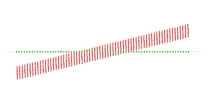
Looking one layer deeper, correction is registration against an “ideal pose”: the target it aligns to is not another measured point cloud but an analytically defined reference (here the \(z=0\) plane). It therefore needs no nearest-neighbor iteration — the target geometry is closed-form, and a single fit yields the transform. Generalize this idea, and aligning to CAD reference planes, reference axes, and reference holes are all the same class of “align to ideal geometry” correction problems.
39.6 SciVision Implementation
The geometry and mathematics of this chapter — kd-tree, Kabsch (SVD), point-to-point / point-to-plane iteration, plane fitting and rotating upright — are all hand-written, and this is precisely the core of the chapter; the SciVision SDK here only plays the supporting role of point-cloud IO and cross-validation evidence. This choice has measured backing: several of this machine’s SDK 3D entry points are simply unreliable in registration scenarios — some overloads of Sci3DKdtree::CreateKdTree return error code 121106105, and Sci3DAxisTransform::Transform3DPointArray crashes outright with 0xC0000005; only SciSv3DSurfaceCorrection::ApplyPlaneCorrection is usable, and this chapter uses it to corroborate the plane-correction result. The sample project runs each SDK probe in a separate subprocess to isolate potential crashes without affecting the main flow’s figure output.
The main loop of nearest neighbor + correspondence rejection (median threshold):
for (size_t i = 0; i < src.size(); ++i) {
    cur[i] = mul(res.R, src[i]) + res.t;   // transform source point by current pose
    nn[i]  = kd.nearest(cur[i], d2[i]);    // hand-written kd-tree nearest neighbor
}
std::sort(sorted.begin(), sorted.end());
double med    = sorted[sorted.size() / 2];           // median of correspondence distances
double thresh = std::max(med * 2.5, 0.5);            // median-method rejection threshold
// keep only correspondences with dist <= thresh for Kabsch -- large-distance intruder-wall pairs are blocked
The filtered correspondences are handed to Kabsch to solve the closed-form rigid transform (centering + cross-covariance SVD + determinant correction), corresponding line by line to the formulas in Section 39.1:
Mat3 H = /* Σ p_i' q_i'^T */;
symEig3(mul(transpose(H), H), w, V);                 // eigendecomposition of H^T H -> right singular vectors
// columns of U = H v_i / σ_i; σ_i = sqrt(λ_i)
Mat3 VUt = mul(V, transpose(U));
double d  = det(VUt) < 0 ? -1.0 : 1.0;               // prevent reflection, force det(R)=+1
R = mul(mul(V, Mat3{{1,0,0, 0,1,0, 0,0,d}}), transpose(U));
t = ct - mul(R, cs);
The point-to-plane variant linearizes each correspondence into a \(6\times6\) normal equation, with the unknowns being the small-angle rotation \(\boldsymbol\alpha\) and the translation:
double r = dot(s - q, nrm);          // signed distance from point to target tangent plane
Vec3   c = cross(s, nrm);            // Jacobian of the rotation part
double a[6] = {c.x, c.y, c.z, nrm.x, nrm.y, nrm.z};
for (int u = 0; u < 6; ++u) {        // accumulate the normal equations A x = b
    for (int v = 0; v < 6; ++v) A[u][v] += a[u] * a[v];
    bb[u] += -r * a[u];
}
Plane correction uses fitPlane (least-squares solution of \(z=ax+by+c\)) to find the normal, then rotateVecToZ (rotation axis \(\mathbf n\times\mathbf z\) + Rodrigues) to rotate upright — two hand-written functions, with SciSv3DSurfaceCorrection as corroboration. The complete runnable project is in code/icp_registration/.
Industry Case: Point Cloud Registration for Robotic Picking
Parts to be picked lie scattered in a bin; the robot relies on a 3D camera to scan a point cloud, register it to the CAD model, solve the 6DoF pose, and then plan the grasp. An early approach used pure ICP directly, and the line crashed again and again — with the parts’ initial poses in disarray, ICP kept falling into wrong local minima, the pose drifted off, and the manipulator grabbed off-target or even grabbed nothing. The key to the overhaul was to add the coarse-registration link: first use the point pair features of 3D matching (Chapter 40) to compute a rough pose, then hand it to ICP to refine to sub-millimeter accuracy, and only then did the pose stabilize. Another unavoidable pitfall is non-overlap: bin walls and neighboring parts both enter the field of view, and these points have no correspondence on the target model and must be blocked one by one by correspondence rejection (distance threshold), or they will drag the pose outward. The lesson: ICP is a refiner, not a searcher; there must always be a coarse registration in front to feed it an initial value.
39.7 Summary
- Registration = solving for the rigid transform \((\mathbf R,\mathbf t)\) that makes two point clouds coincide, the 3D upgrade of 2D position correction (Chapter 19); ICP uses the loop “find correspondences by nearest neighbor → reject far correspondences → solve the optimal transform by SVD → iterate” to break the deadlock in which correspondence and transform are each other’s cause and effect.
- Kabsch / Umeyama gives the closed-form optimal rigid transform: subtract the centroid, construct the cross-covariance matrix \(\mathbf H\), take its SVD, \(\mathbf R=\mathbf V\,\mathrm{diag}(1,1,d)\,\mathbf U^\top\), where \(d\) prevents degeneration into a reflection — this is a direct application of the SVD from Chapter 2.
- ICP only guarantees local convergence and is highly sensitive to the initial value: with a good initial value it converges in 58 iterations to RMS 0.6443 mm; with a bad initial value (an extra \(40°\) rotation) it falls into a wrong local minimum, with rotation error 29.3°. Industry must go coarse-to-fine — first use 3D matching (Chapter 40) for coarse registration to supply the initial value, then use ICP to refine.
- The point-to-plane variant is far faster than point-to-point: penalizing only normal deviation and letting tangential sliding pass, this chapter’s experiment reaches RMS 0.0991 mm in 9 iterations (point-to-point still stops at 0.6443 mm after 58), so industrial ICP mostly adopts point-to-plane.
- 3D correction is registration against an “ideal pose”: fit a reference plane + rotate upright to \(+Z\), dropping a 7° tilt to 0.0000° in one step; non-overlap (intruder walls, bin walls) must be blocked by correspondence rejection, a prerequisite for registration to land reliably.
For a more systematic treatment of ICP, point cloud registration, and 3D pose estimation, see the book by Steger et al. (Steger, Ulrich, and Wiedemann 2018). The ICP algorithm itself has two classic origins: Besl and McKay gave the point-to-point formulation based on iterating to the closest point (Besl and McKay 1992), while Chen and Medioni, registering multiple range images, proposed the faster-converging point-to-plane error metric (Chen and Medioni 1992) — exactly the 58-vs-9-iteration difference in this chapter’s experiments; a systematic comparison of the sampling, matching, and rejection variants is given in the survey by Rusinkiewicz and Levoy (Rusinkiewicz and Levoy 2001). Each round’s closed-form optimal rigid transform, obtained by the SVD of the cross-covariance matrix after centroid subtraction (Kabsch/Umeyama), was first rigorously derived in the paper by Arun, Huang, and Blostein (Arun, Huang, and Blostein 1987).