4 Illumination

There is an old saying in the machine vision industry: “Half of a vision project’s success or failure is decided by the lighting.” This is no exaggeration: cameras and algorithms deal in gray values, and gray-value differences are the product of the interaction between illumination and the surface. A scratch, a missing piece of material, a row of characters — each only images as a separable gray-value difference under the right illumination. If the lighting fails to pull the target apart from the background, no algorithm, however ingenious, can make bricks without straw. Conversely, one well-chosen lighting setup often reduces the algorithm from elaborate texture analysis to a single threshold segmentation.

This chapter answers two questions. First, faced with a new inspection target, how do you choose the illumination — bright field or dark field, front lighting or backlight, which color? Second, what are the consequences of non-uniform illumination, and what are the two remedies: flat-field calibration on the hardware side and shading correction on the software side. The second half comes with a complete quantitative experiment.

4.1 Illumination Modes and Selection

The core variable of an illumination mode is the relationship between the light’s angle of incidence and the lens’s viewing angle. If the specular reflection from the surface enters the lens directly, the background is lit up — this is bright-field illumination. If only the light scattered by surface relief enters the lens, the flat background stays dark while raised or recessed features light up — this is dark-field illumination. The same scratch appears as a faint dark streak on a bright background in bright field, but as a bright thin line on a black background in dark field — the contrast can differ by an order of magnitude. Classified by position along the optical path, there is also front lighting, illuminating from the camera side, and backlight, illuminating from behind the target; the latter images the target’s outline as a clean black silhouette. Common modes and their typical applications are summarized below.

Illumination mode	Working principle	Suitable surfaces and defect types
Bright-field front light	Reflected light enters the lens; background is bright	Printing, characters, stains on diffuse flat surfaces
Low-angle ring light / dark field	Grazing-angle illumination; only scattered light from relief enters the lens	Scratches, burrs, dents, edge chipping
Backlight	Outline imaged as a black silhouette	Outer dimensions, hole diameters, lead-pitch measurement
Coaxial light	A half-mirror sends light out along the optical axis	Highly reflective flat surfaces: glass, wafers, polished metal
Diffuse dome	All-angle diffuse light, eliminating highlights	Curved and uneven metal: can bottoms, solder balls

Color is a design variable too. In monochrome inspection, a complementary color is often used to boost contrast: red printing appears nearly black under green light, yet all but vanishes under red light. Industrial sites favor red LEDs — not only because the devices are mature and cheap, but because paired with a narrow-band filter they effectively reject ambient light: shop-floor ceiling lights and daylight through skylights are all filtered out, and the image is determined solely by the controlled source. Incidentally, pushing the dark-field idea of “using lighting direction to reveal surface relief” to its extreme yields photometric stereo, which uses sources from multiple directions to solve back for the surface normals (Chapter 34).

The lighting-experiment method: run a sample trial before choosing an algorithm. When a new workpiece arrives, the first thing to do is bring several typical light sources (ring, bar, coaxial, backlight) and test-shoot the sample with each one, picking the combination with the highest defect contrast and the cleanest background — only then start thinking about algorithms. An hour of experiments at the illumination stage often saves a month of struggle at the algorithm stage.

4.2 The Harm of Non-uniform Illumination

Even with the right illumination mode chosen, the spatial uniformity of the illumination can still go wrong. Non-uniformity has two major sources. The first is vignetting: a lens’s natural light falloff follows the \(\cos^4\theta\) law — illuminance decays with the fourth power of the cosine of the off-axis angle (\(\cos^4\theta\)) — and, combined with mechanical obstruction by the lens barrel, the corners of the frame are inherently darker than the center. The second is source geometry: unequal distances from the source to the surface, single-sided lighting, and unevenly aged LED beads all superimpose lateral brightness gradients. The result is that the same kind of surface shows different gray values at different positions in the image — which breaks precisely the implicit assumption behind most algorithms.

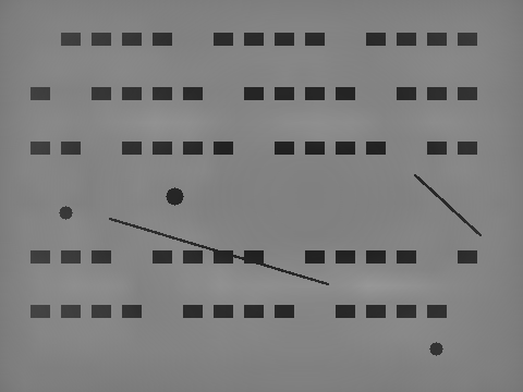
We quantify this with a synthetic experiment. The ideal scene is \(480\times360\) pixels: on a uniform background of gray value 160, there are five rows of text-like dark bands, three defect blobs, and two thin scratches 2 px wide, all targets at gray value 60. We then overlay a synthetic non-uniform illumination field: a radial falloff toward the corners of \(1-0.45(r/r_{\max})^2\) (45% light loss at the corners), multiplied by a horizontal gradient from \(0.9\) to \(1.1\) simulating a single-sided source bias. The two images are shown in Figure 4.1.

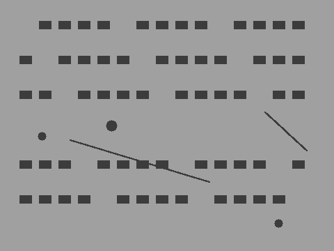
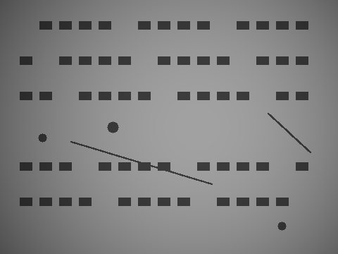
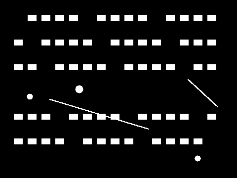
Note that to the human eye Figure 4.1 (b) does not look too bad — the targets are still clearly visible. But an algorithm is not a human eye. With background at 160 and targets at 60, take the midpoint \(T=110\) as a fixed threshold (pixels darker than \(T\) classified as target): on the ideal image the misclassified pixels number 0; on the vignetted image, the misclassified pixels soar to 16327 — about 9.4% of the image’s 172800 pixels. The results are shown in Figure 4.2.

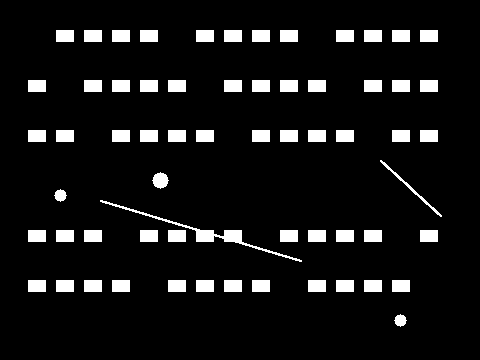
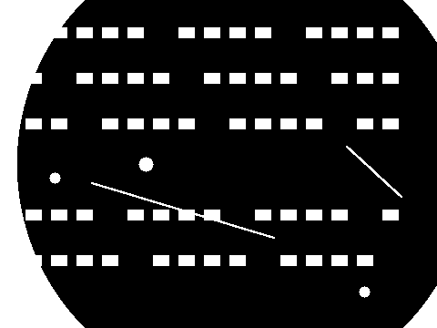
(a) Ideal image binarized: 0 misclassified

The failure mode deserves a close look: the two left corners are pressed down by the gain field to about 88 and the two right corners to about 106 — all below the threshold of 110, flipping wholesale into “target”; meanwhile the real marks lying in the corners are swallowed by these misclassified regions and can no longer be separated out. This is not a gradual degradation of “accuracy dropping a few percentage points” but total failure — the global threshold’s premise, “the same kind of surface has the same gray value everywhere,” is destroyed outright by the illumination. There are two classes of remedy: on the algorithm side, switch to locally adaptive thresholds (see Chapter 7); on the illumination side, cure the non-uniformity itself. This chapter takes the second route.

4.3 Flat-Field Calibration and Software Correction

There are two routes to curing non-uniform illumination, corresponding to the “with reference” and “without reference” working conditions.

Route one: flat-field calibration. Place a uniform white board (or a diffuse reflectance standard) on the line and capture one image — the board itself has the same gray value everywhere, so the light-and-dark variation in the captured image is purely the gain field of the illumination and the lens. In this experiment we apply the same gain field to a blank target of gray value 200; the resulting flat-field reference image is shown in Figure 4.3.

Figure 4.3: Flat-field reference image: imaging a uniform white board, the resulting brightness distribution is the pure gain field of the illumination system — dark on the left and bright on the right, dark in the corners and bright in the center, exactly the same structure as Figure 4.1 (b).

With the flat-field reference image \(F\), correction is a single per-pixel division:

\[ g_{\text{corr}}[n,m] = \frac{g[n,m]}{F[n,m]}\,\bar F, \]

where \(\bar F\) is the mean of \(F\); multiplying it back keeps the corrected image at its original overall brightness level. Once the gain field is divided out, the illumination non-uniformity vanishes at its source. Flat-field calibration is the production line’s first choice: physically rigorous and computationally cheap. Its cost is that it requires a reference image — it must be redone after a lens change, an aperture change, or light-source aging — and some stations (continuous in-line motion, large fields of view) simply cannot accommodate a white board.

A more rigorous flat-field calibration also subtracts the dark frame — capture one image with the lens cap on to obtain the sensor’s fixed offset: \(g_{\text{corr}} = (g-D)/(F-D)\cdot\overline{(F-D)}\). For industrial 8-bit cameras the offset is tiny and often omitted; for scientific-grade cameras and long exposures it must not be.

Route two: shading correction with self-estimated background. When no reference image is available, the illumination distribution can be estimated from the image itself: illumination variation is large-scale (a slow drift spanning the whole frame), while target structures are small-scale (characters a dozen-odd pixels tall, scratches a few pixels wide) — the two are separable in spatial scale. Low-pass filter at a sufficiently large scale (echoing Chapter 6, except that here the low-frequency component is treated as the “illumination layer” to be removed rather than the signal to be kept) so that the small targets are flattened away, and what remains is an estimate of the background illumination; then normalize the original image against this background, and the correction is done. The precondition follows immediately: the targets must be significantly smaller than the scale of the illumination variation — if the defect itself is a large gradual patch (such as a large-area color deviation), it will be wiped out along with the illumination.

We use the SciVision SDK’s shading correction (parameters detailed in Section 4.4) to process Figure 4.1 (b); it is exactly an implementation of self-estimated background and needs no flat-field reference image. The results are shown in Figure 4.4.

Quantitatively, comparing the mean gray value of \(20\times20\) background patches at the four corners and the center:

Table 4.1: Mean gray values of background patches at the four corners and the center: correction compresses a spatial range of 72 levels down to 4.5 levels

Image	Top-left	Top-right	Bottom-left	Bottom-right	Center	Range
Ideal illumination	160.0	160.0	160.0	160.0	160.0	0
Vignetted	87.6	105.9	87.6	105.9	159.9	72.3
Corrected	125.4	125.2	125.4	124.5	129.0	4.5

The background range converges from 72 levels to 4.5 levels. Note that the corrected level is about 125 rather than the original 160 — what software correction guarantees is “flat,” not “restored to the original value”; and for threshold segmentation, flat is enough. Under the same threshold \(T=110\), the misclassified pixels drop from 16327 to 0 — pixel-for-pixel identical to the segmentation under ideal illumination.

An early version of this experiment reported “221 residual misclassifications after correction, all on the outermost 1 px ring” and misattributed them to the SDK leaving the outermost rows and columns unprocessed. A later audit found the root cause on the calling side: the bottom-right corner of SciROI::GenRect1 is an exclusive endpoint, and the \((W-1,H-1)\) passed at the time excluded the last row and column from the ROI. After passing \((W,H)\) to cover the full image, the residual misclassifications vanish to 0.

4.4 SciVision Implementation

Shading correction is provided by the SCIMV::SciSvShadingCorrection class; the call used in this chapter’s experiment is identical to the accompanying project code:

SCIMV::SciSvShadingCorrection sc;
SciImage dst;
long rc = sc.CorrectShading(src, roi,
    2,      // lightOrDark=2: keep both bright and dark targets (flatten background only)
    1.0,    // gain: gain of 1, no extra contrast amplification
    15,     // extractSize: extraction size, slightly larger than the target block height (text blocks are 12 px tall)
    2,      // correctionMethod=2: shading correction
    0,      // filterValue: do not exclude interfering gray values
    0,      // direction=0: both X and Y directions
    5,      // filterkernelSize: background-estimation filter kernel
    &dst);

The meaning of each parameter and the rationale for its value are as follows.

lightOrDark: specifies whether to keep targets brighter than the background, darker than it, or both; 2 means both bright and dark targets are kept, and the correction touches only the background.
gain: the contrast gain after correction; 1.0 means no extra stretching. It can be raised moderately when the targets’ own contrast is weak.
extractSize: the structure scale removed as “foreground” during background estimation; 15 is slightly larger than the 12 px text-block height, which together with the filtering is sufficient. Set it too small and the targets get mistaken for background and wiped out.
correctionMethod: must be 2 (shading correction). In our tuning trials we observed (that sweep is not included in the accompanying project) that 0 (median) or 1 (mean) performs only a global level normalization — the whole image is shifted to one common mean, the corners stay dark, and the spatial non-uniformity does not budge.
filterValue: excludes interfering pixels of a specified gray value; 0 means no exclusion.
direction: the direction of the background gradient. In the tuning trials we observed that 1 (X only) or 2 (Y only) can also flatten the numbers, but a single-direction background estimate folds the target bands of the other direction into the background, leaving visible striping artifacts across the text bands; 0 (both X and Y) is the cleanest.
filterkernelSize: the smoothing kernel for background estimation; a small kernel (5) combined with both directions is already sufficient. The larger the kernel, the smoother the background — but also the larger the background-estimation bias near large targets.

The complete project that generates all of this chapter’s images and statistics is located at code/illumination/; you can modify the gain-field strength and each parameter to reproduce the parameter-sweep conclusions above.

Industry Case: An Illumination Faceplant in Glass Scratch Inspection

A cover-glass inspection project initially used bright-field front lighting: the glass surface reflected the light evenly into the lens, scratches caused a disturbance of only about 5 gray levels, the detection rate was below thirty percent, and for a while the team tried to brute-force it with elaborate texture-enhancement algorithms. The setup was then switched to a low-angle dark-field ring light: the flat glass surface scatters nothing toward the lens, so the background goes nearly black while scratches scatter into bright lines; the contrast rose above 80 levels, and the algorithm collapsed to a single threshold segmentation. But dark field brought a new problem of its own — at grazing angles the illuminance is extremely sensitive to distance and angle, the background at the edges of the field of view turned visibly gray, and the fixed threshold kept raising false alarms in the edge regions. Only after layering this chapter’s software shading correction on top to flatten the background did the system truly stabilize. Two lessons: illumination and algorithm are one system and must be designed together; and every doubling of contrast won by the lighting saves algorithm complexity by a factor of ten.

4.5 Summary

Illumination determines the gray-value difference, and the gray-value difference sets the ceiling for the algorithm. Selection rule of thumb: diffuse surfaces — bright field; scratches and burrs — dark field (low angle); outlines and dimensions — backlight; highly reflective flats — coaxial; curved glossy surfaces — dome. Run a sample trial first, then fix the algorithm.
Non-uniform illumination (vignetting + lateral gradient) makes a global threshold fail outright, not degrade gradually: in this chapter’s experiment, the fixed threshold’s misclassifications shot from 0 to 16327 pixels, with whole patches of corner background flipping over.
Flat-field calibration divides out the gain field per pixel using a white-board reference image (\(g/F\cdot\bar F\)); physically rigorous and computationally cheap, it is the first choice whenever a reference board can be placed. It must be redone after a lens change, an aperture change, or light-source aging.
Software shading correction estimates the background from the image itself with a large-scale low-pass filter and then normalizes — no reference image needed; the precondition is that target scale is far smaller than the illumination-variation scale. In this chapter’s experiment the background range was compressed from 72 levels to 4.5, and misclassifications fell from 16327 to 0 (note that the bottom-right corner of GenRect1 is an exclusive endpoint: a full-image ROI must be passed as \((W,H)\)).
The parameters are not black magic: correctionMethod must be set to shading correction (0/1 only do global normalization), a single-direction direction leaves striping artifacts, and extractSize must be slightly larger than the largest target — all reproducible, measured conclusions.

For a systematic treatment of illumination engineering and radiometric calibration, see further the book by Steger et al. (Steger, Ulrich, and Wiedemann 2018). This chapter’s flat-field calibration and shading correction address spatial non-uniformity, whereas the nonlinear response between gray value and scene irradiance — the camera response function — must be calibrated separately: Mitsunaga and Nayar (Mitsunaga and Nayar 1999) introduced radiometric self-calibration, recovering the response curve from a few differently exposed images without any reference radiance source, a foundation for accurate photometry and HDR imaging. To instead exploit controlled illumination actively to extract information, Woodham’s (Woodham 1980) photometric stereo solves per-pixel surface normals from several images taken under known, varying light directions from a single viewpoint — the classic paradigm of “active lighting for measurement”.