35 Phase Measuring Deflectometry
Put a piece of polished phone cover glass, a mirror-finished stainless-steel panel, or a plane mirror onto the production line, and the 3D imaging techniques built up in the preceding chapters fail en masse: the fringes projected by structured light (Chapter 32) no longer diffuse back to the camera but are reflected straight off to somewhere else by the specular surface; laser triangulation (Chapter 30) cannot find a stable scattered light stripe; binocular stereo has nothing to match either — what you see on a mirror is not surface texture at all, but a reflection of the surroundings. Light does not diffuse on a mirror, so every method that relies on “seeing the surface lit up” loses its footing.
Yet a mirror can do precisely one thing other surfaces cannot: serve as a mirror. If we let the specular surface reflect a screen displaying sinusoidal fringes, what the camera sees “in the mirror” is fringes distorted by the surface relief. Wherever the surface tilts a little, the fringes reflected into the camera shift a little there — the amount of fringe distortion directly encodes the surface slope. This is phase measuring deflectometry (PMD): instead of illuminating the surface to measure height, it treats the surface as a reflecting mirror and infers slope from the phase shift of the fringes. Figure 35.1 is the raw image obtained from the surface under test reflecting the screen fringes, where the shallow bump and the scratch-like groove have already left visible local distortions on the regular fringes.
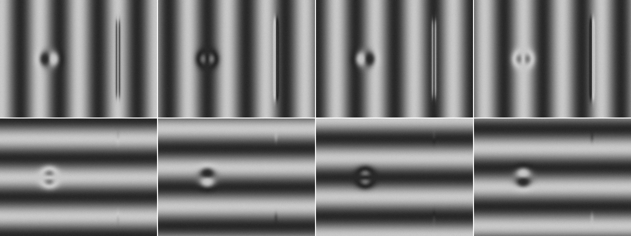
PMD and structured light (Chapter 32) are a dual pair: structured light requires the surface to be diffuse and measures height directly; PMD requires the surface to be specular and measures slope directly. The two use the very same phase-shifting and unwrapping machinery, yet serve two geometrically opposite classes of surface. Almost every property in this chapter has its mirror image in the structured-light chapter.
35.1 Specular Reflection and Slope Encoding
The geometry of PMD is made up of three players: the screen that emits the fringes, the specular surface under test that reflects the fringes into the camera, and the imaging camera. The screen displays a spatial sinusoidal pattern at distance \(L\) from the surface; each line of sight from the camera hits a point on the surface, folds back to the screen according to the law of reflection, and lands at some screen coordinate — the screen phase at that coordinate is the phase observed by that pixel.
The key is how a surface tilt changes this light path. Let the local slope of the surface at some point be \(s=\partial h/\partial x\), i.e. the surface is tilted by a small angle \(\alpha\approx s\) relative to the reference plane. The law of reflection tells us: if the surface normal rotates by \(\alpha\), the reflected ray rotates by \(2\alpha\) — this is the factor-of-2 deflection law of deflectometry. The lateral landing point of the ray at screen distance \(L\) is therefore shifted by about \(2L\tan\alpha\approx 2L\,s\). So what the camera observes at that pixel is no longer the phase of the screen point straight below, but the phase of the point shifted by \(2L\,s\):
\[ \varphi_{\text{obs}}(x)\;\approx\;\varphi_{\text{screen}}\!\big(x + 2L\,\tfrac{\partial h}{\partial x}\big). \]
The “factor of 2” comes from the law of reflection: turn the mirror by \(\alpha\), the ray turns by \(2\alpha\). This is also why PMD is so exquisitely sensitive to slope — a milliradian tilt of the surface is magnified at \(L=200\) mm away into a fringe displacement of \(2L\alpha=0.4\) mm, equal to 2.5% of the fringe period \(P=16\) mm, clearly distinguishable in phase. The geometry carries a first stage of amplification built in.
Subtracting from it the uniform screen phase \(\varphi_{\text{screen}}(x)=2\pi x/P\), the offset of the observed phase relative to the plane-mirror reference is proportional to slope: \(\Delta\varphi = \varphi_{\text{obs}}-\varphi_{\text{ref}} = (2\pi/P)\cdot 2L\,s\). In other words,
\[ s \;=\; \frac{\partial h}{\partial x} \;=\; \frac{P}{2\pi\cdot 2L}\,\Delta\varphi . \]
This equation is the root of all of PMD’s properties: it measures slope \(\partial h/\partial x\), not height \(h\). Height can only be obtained indirectly by integrating the slope field (Section 35.3). This stands in sharp contrast to structured light — the phase of structured light is directly proportional to height, while the phase of PMD is proportional to the derivative of height. The derivative is sensitive to high-frequency relief and sluggish about absolute magnitude, and this trade-off runs through the whole chapter: it makes PMD astonishingly sensitive when detecting tiny relief (Section 35.4), yet also makes the absolute height depend on a drift-prone integration.
35.2 Reusing Phase Measurement
Since the measured quantity is the phase of the screen fringes, the machinery for recovering phase can be borrowed wholesale from structured light (Section 32.1). The screen displays 4-step phase-shifted fringes along x, the camera captures 4 frames \(I_0\ldots I_3\), and the wrapped phase is computed by hand with the four-step phase-shift formula:
\[ \varphi_{\text{wrap}} = \operatorname{atan2}\!\big(I_3-I_1,\; I_0-I_2\big), \]
As in the structured-light chapter, SciVision’s SciSvPhaseMeasure::DecodePatterns (four-step phase-shift decoding) is inert in this SDK build — it returns code 0 but outputs an empty image. PMD is exactly its home turf, so the example still probes it once more with genuine bidirectional X+Y fringes and faithfully records its failure, after which the entire phase pipeline is written by hand (wrapped phase via atan2 + spatial unwrapping).
The modulation \(B=\tfrac12\sqrt{(I_3-I_1)^2+(I_0-I_2)^2}\) measures the fringe contrast along the way, to be used later in Section 35.5. Because the deflection phase field is smooth (carrier about 0.08 rad/px, and the deflection introduced by a defect is well under \(\pi\)), single-frequency spatial unwrapping on a flat mirror is enough — no need for the dual-frequency hierarchical method of structured light (Section 32.2). One pass each for x and y yields the unwrapped phase in both directions.
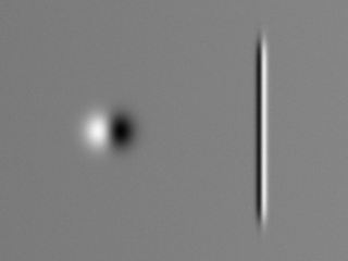
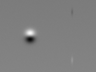
The final step of measurement is to subtract the plane-mirror reference phase: render a separate set of phase-shifted images of an ideal plane mirror, solve for its phase \(\varphi_{\text{ref}}\), and subtract it from the measured phase to cancel the carrier and the system geometry; the remaining \(\Delta\varphi\) converts directly into the slope fields \(s_x,\,s_y\). Figure 35.2 is the slope map in the two directions. The most intriguing feature is the bipolar signature of the bump in the x-direction slope map (Figure 35.2 (a)): a 50 μm Gaussian bump appears on the slope map not as a single bright blob, but as two lobes, one positive and one negative — because slope is the derivative of height, the up-slope of the bump is positive and the down-slope negative, with the slope crossing zero at the peak. In the measured neighborhood of the bump the x-direction slope swings between \(-0.0146\) and \(+0.0141\) rad, agreeing with the theoretical peak slope \(\pm 0.0143\) rad of the Gaussian bump. The scratch-like groove on the right, extending along y and having slope only in x, shows up as a clean vertical line.
35.3 Slope Integration and Height
To obtain height, one must integrate the slope field back up — this is isomorphic to recovering height from the normal field in photometric stereo (Chapter 34): both hold the surface gradient and both need to recover a scalar height field. The most naive approach is to accumulate a trapezoidal integral along a path: integrate \(s_y\) down the first column, then integrate \(s_x\) row by row to get the height along one path; switch to another path (first \(s_x\) along the first row, then \(s_y\) column by column) and compute again, averaging the two paths to suppress noise. With a smooth surface and small noise, this simple integrator does the job without the complexity of a Poisson solver.
Integration has an inherent weak spot: low-frequency drift. Slope noise accumulates along the integration path and piles up into a slowly undulating “terrain” on the height map; together with the integration constant itself being undetermined, PMD’s absolute height and large-scale form are not reliable. This is exactly where it is complementary to structured light — structured light has accurate absolute height but poor high-frequency sensitivity; PMD is the reverse.
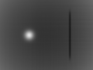
Figure 35.3 is the height map obtained by integration. Quantitatively, the example measures the bump height as 46.83 μm using the central disk minus an outer-ring baseline (GT 46.71, nominal 50), and the groove depth as 10.13 μm using the groove bottom minus a side baseline (GT 10.16, nominal 10) — both close to the true values, with the residual deviation coming mainly from the finite-aperture baseline selection rather than measurement noise. The height RMS error in the flat region is only 0.228 μm: slope integration spatially averages the per-pixel noise, compressing the \(1.6\times10^{-4}\) rad slope noise down to sub-micron height noise.
35.4 Sensitivity: Why Measuring Slope Is So Accurate
This is the heart of the chapter. PMD measures slope, and slope is an angle — angular quantities are extremely easy to measure precisely, because the screen distance \(L\) magnifies a tiny tilt into a sizable fringe displacement. Working through the noise derivation makes this clear. The phase noise of four-step phase shifting is \(\sigma_\varphi=\sigma_N/(\sqrt2\,B)\); subtracting the reference from the measurement amplifies it by another \(\sqrt2\), giving \(\sigma_{\Delta\varphi}=\sigma_N/B\), so the slope noise is
\[ \sigma_{\text{slope}} \;=\; \frac{\sigma_N}{B}\cdot\frac{P}{2\pi\cdot 2L}. \]
Substituting \(\sigma_N=2,\,B=80,\,P=16\) mm\(,\,L=200\) mm, the theoretical value is \(\sigma_{\text{slope}}=1.592\times10^{-4}\) rad, consistent with the measured \(1.643\times10^{-4}\) rad. Just how small is this angular noise? For a defect of base width \(w\) and height \(h\), the maximum slope is about \(4h/w\); the condition for it to be detectable is that this slope exceed the noise, i.e. \(4h_{\min}/w\approx\sigma_{\text{slope}}\), giving the minimum detectable height
\[ h_{\min}\;\approx\;\frac{\sigma_{\text{slope}}\,w}{4}. \]
Substituting the measured \(\sigma_{\text{slope}}\): a \(w=1\) mm defect gives \(h_{\min}=0.041\) μm, \(w=5\) mm gives 0.205 μm, and \(w=20\) mm gives 0.821 μm. Narrow, shallow microscopic defects can be measured down to tens of nanometers — far beyond the reach of methods that measure height directly.
The comparison is right there in Figure 35.4. The same surface and the same 50 μm bump: the left image is the PMD slope map, the right is what structured light sees at its height noise floor (measured at 33.8 μm in ch32). The structured-light height noise floor is almost on the same order as the 50 μm bump, so the bump is drowned in granular noise and barely discernible; on the PMD slope map, by contrast, the bump and the groove are strikingly clear. Quantitatively: for the same bump, the PMD slope SNR is 87:1, while the structured-light height SNR is only 1.5:1, a difference of about 59×.
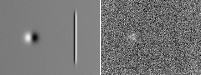
There is no free sensitivity. PMD is exquisitely sensitive to slope (high-frequency relief), at the cost of an absolute height that depends on a drift-prone integration (Section 35.3) and is, conversely, sluggish about slow large-scale undulations. Structured light is exactly the opposite. In engineering the two are often complementary: structured light fixes the large-scale form, PMD fills in the microscopic high-frequency defects.
35.5 The Boundary of Specularity
The entire premise of PMD is specular reflection. Once the surface turns rough, the microfacets scatter the incident light, and the contrast of the specularly reflected fringes collapses accordingly. The example sweeps roughness through the diffuse fraction \(\rho\), convolving the screen sinusoidal pattern with a Gaussian scattering lobe, so that the effective contrast decays as \(B_{\text{eff}}=(1-\rho)B\exp[-\tfrac12((2\pi/P)\cdot2L\,\sigma_\theta)^2]\), and the phase noise \(\propto 1/B\) explodes along with it:
| \(\rho\) | Contrast \(B\) | Phase RMS (rad) | Slope RMS (rad) | \(h_{\min}\) (w=5mm, μm) |
|---|---|---|---|---|
| 0.0 | 80.0 | 0.0255 | \(1.626\times10^{-4}\) | 0.203 |
| 0.3 | 47.7 | 0.0364 | \(2.314\times10^{-4}\) | 0.289 |
| 0.7 | 10.1 | 0.1449 | \(9.222\times10^{-4}\) | 1.153 |
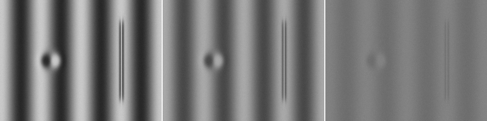
From \(\rho=0\) to \(0.7\), the contrast collapses from 80 to 10, the phase RMS rises by nearly 6×, and the minimum detectable height degrades from 0.20 μm to 1.15 μm. The three fringe images of Figure 35.5 make this collapse vividly clear: in the left image the fringes are crisp and the defect is distinct, while by the right image the fringes have turned into a hazy gray and the signal is all but buried. This is precisely the mirror dual of the modulation story (Section 32.4) of the structured-light chapter — structured light requires the surface to be diffuse enough and fails in specular regions due to specular-highlight saturation; PMD requires the surface to be specular enough and its contrast collapses as soon as the diffuse component grows. A semi-specular surface is a dilemma for both: too bright and the mirror does not move, too rough and the diffuse signal is insensitive, and surfaces landing in this middle ground tend to give both methods trouble.
35.6 SciVision Implementation
The entire PMD pipeline reuses the phase machinery of ch32. As covenanted, SciSvPhaseMeasure::DecodePatterns is still inert in PMD, its very home turf (returns 0, outputs an empty image), so the example probes it once more with a genuine bidirectional X+Y fringe set, faithfully records its failure, and then writes everything by hand. The key slope-extraction and integration snippet follows.
// 1. Four-step phase-shift wrapped phase (one set each for x/y),
//    subtract the plane-mirror reference phase -> slope field
double s = (double)im[3][i] - im[1][i];   // 2B*sin(phi)
double c = (double)im[0][i] - im[2][i];   // 2B*cos(phi)
phi[i]   = std::atan2(s, c);              // wrapped phase
// after unwrapping: dphi = phi_obs - phi_ref, convert to slope (rad)
//   via the factor-of-2 deflection law
slope[i] = (uObs[i] - uRef[i]) * P_SCR / (TWO_PI * 2.0 * L_SCR);

// 2. Two-path trapezoidal integration of slope -> height
//    (same form as photometric-stereo normal integration)
h1[i] = h1[i-1] + 0.5 * (sx[i] + sx[i-1]) * PX;   // path 1: integrate sx row by row
h2[i] = h2[i-W] + 0.5 * (sy[i] + sy[i-W]) * PX;   // path 2: integrate sy column by column
h[i]  = 0.5 * (h1[i] + h2[i]);                    // average the two paths to suppress noise
The P_SCR/(TWO_PI*2.0*L_SCR) term in the slope conversion is exactly \(P/(2\pi\cdot2L)\), translating the deflection phase difference into slope; the integration step PX is the physical pixel scale. One calibration point: the geometric accuracy of PMD hinges on the relative poses of screen, camera, and reference plane — the screen-to-surface distance \(L\), the physical scale of the screen pixels, and the camera intrinsics all need to be calibrated beforehand (echoing Chapter 5), and any error in any of them propagates linearly into the slope through the deflection law. The complete project that generates all the images in this chapter is located at code/deflectometry/.
Industry Case: Micro-Defects on Phone Cover Glass
What needs to be inspected on polished phone cover glass is sub-micron microscopic relief: orange peel, polishing marks, shallow scratches, whose height undulations are often only a few tenths of a micron. Measuring height directly with structured light, the height noise floor on the order of 33 μm buries these defects completely, leaving nothing to discriminate; switching to PMD to measure slope, the geometric factor-of-2 deflection law plus the magnification of the screen distance amplifies the sub-micron high-frequency relief into a clearly discernible slope signal, and the defects become obvious at a glance. But the cover glass is not specular everywhere: the chamfered edges and the silk-screened ink regions are diffuse or semi-specular, where the fringe contrast collapses and the phase noise explodes — they must be masked out separately and processed apart, not lumped together with the specular regions. The lesson is direct: for microscopic-relief inspection of specular or mirror-like surfaces, PMD’s slope sensitivity is something structured light cannot give; but PMD’s Achilles’ heel is also its specularity — non-specular regions must first be identified, then isolated.
35.7 Summary
- PMD uses the mirror as a mirror: it lets the specular surface under test reflect the screen fringes and infers surface slope from the fringe phase shift — the remedy precisely for the mirror objects on which structured light, laser, and binocular stereo all fail, and the geometric dual of structured light.
- The factor-of-2 deflection law is the root of everything: a surface tilt \(\alpha\) deflects the reflected ray by \(2\alpha\), \(\varphi_{\text{obs}}\approx\varphi_{\text{screen}}(x+2L\,\partial h/\partial x)\). PMD measures slope rather than height; height requires integrating the slope field (isomorphic to photometric stereo), at the cost of a drift-prone absolute height.
- Measuring slope makes it exquisitely sensitive: \(h_{\min}\approx\sigma_{\text{slope}}w/4\), only 0.205 μm at \(w=5\) mm. For the same 50 μm bump, the PMD slope SNR of 87:1 versus the structured-light height SNR of 1.5:1 is about a 59× gain — PMD amplifies high-frequency relief.
- Specularity is a hard boundary: as the surface roughens, the fringe contrast collapses and the phase noise explodes (\(h_{\min}\) degrades 5× at \(\rho=0.7\)), the mirror image of the structured-light modulation story; a semi-specular surface is troublesome for both methods.
- Reuse the phase machinery, mind the calibration: phase shifting and unwrapping follow ch32 (
DecodePatternsinert, written by hand), and the accuracy hinges on the screen-camera-reference-plane geometric calibration.
The pioneering work on measuring specular free-form surfaces with phase measuring deflectometry is the paper by Knauer, Kaminski, and Häusler (Knauer, Kaminski, and Häusler 2004); the principles, calibration, and application advances of the field are comprehensively surveyed by Huang et al. (Huang et al. 2018). The engineering treatment of deflectometry and 3D measurement of specular surfaces can be further consulted in the book by Steger et al. (Steger, Ulrich, and Wiedemann 2018).