23 Blob Analysis
Thresholding (Chapter 7) turned the image into black and white, but the question the production line asks is never “which pixels are white?” — it is: how many chip components are on this tray? Which of them are touching each other and need to be re-fed for rework? How big is the largest blob, and where is it? To answer such questions, we must first organize “a heap of white pixels” into “individual objects” — this is the first stop after segmentation. Blob analysis = connected component extraction + feature computation + filtering and classification; together these three steps form the backbone of counting, sorting, foreign-object detection, and a good half of the inspection world.
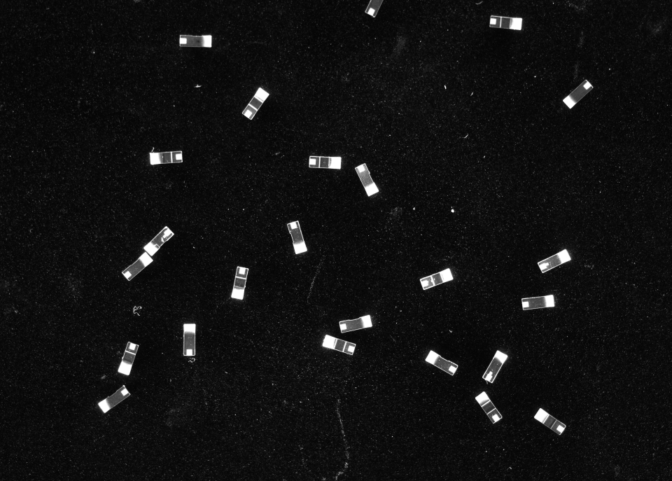
Throughout this chapter, one real industrial sample drives all the experiments (Figure 23.1): a frame from Smart3’s “blob-analysis example recipe” — a batch of surface-mount chip components scattered over a dark felt tray, their metallized end-faces glinting bright under coaxial light. The original image is 3840×2748 single-channel grayscale, box-downsampled ×4 to 960×687 to fit the book figures. Roughly 24 components lie in the field at assorted angles, including one pair touching end-to-end and one component clipped by the bottom field edge; the felt tray, meanwhile, raises a sheet of fine specks under a bright threshold. Our task is to count the components and pick out the touching pair — and every pitfall we hit along the way is a regular visitor on real production lines.
23.1 Connected Components and Labeling
What we call an “object” in a binary image is mathematically a connected component: a set of foreground pixels in which any two can reach each other through a chain of adjacent foreground pixels. The crux lies in the definition of “adjacent” — 4-connectivity recognizes only the four neighbors above, below, left, and right, while 8-connectivity also counts the four diagonal neighbors.
This seemingly trivial choice has very real consequences. Two patches that touch only at a single diagonal corner are one object under 8-connectivity but two under 4-connectivity; a one-pixel-wide diagonal line is a single intact line under 8-connectivity but shatters into a string of isolated points under 4-connectivity. In counting, choosing the wrong connectivity makes the count systematically too high or too low. Industrial libraries almost universally default to 8-connectivity, because the slanted boundaries of real targets, once sampled, naturally connect along the diagonals.
Diagonal contact counts as one blob under 8-connectivity. The touching pair later in this chapter is a different matter, though — those two components physically overlap end-to-end, their pixel sets genuinely merge, and they coalesce under both 4- and 8-connectivity. Another classic convention: when the foreground uses 8-connectivity, the background should use 4-connectivity (and vice versa); otherwise the inside and outside of a closed 8-connected curve would themselves be 8-connected — a topological self-contradiction.
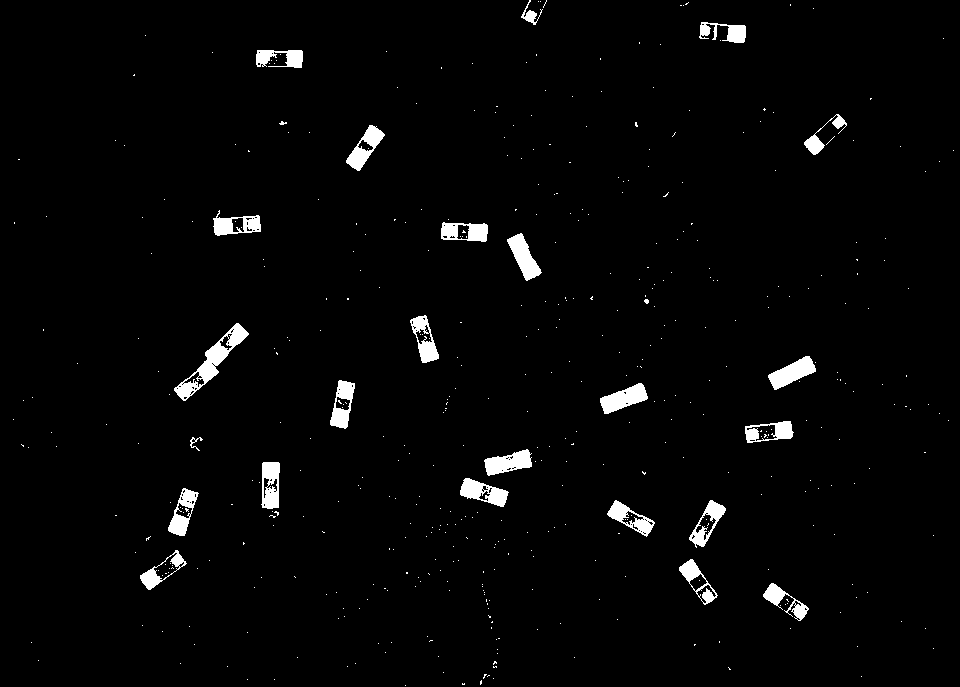
The process of finding each connected component and assigning it a number is called connected component labeling. The classic approach is a two-pass scan: the first pass walks through the rows assigning provisional labels to foreground pixels while recording equivalences (“these labels are actually connected”); the second pass merges the equivalent labels into final numbers. Implementations based on run-length encoding are more efficient — each row’s consecutive foreground segments are first compressed into runs, then connectivity is established between runs on adjacent rows, so the complexity depends only on the number of runs, not on the area. SciVision’s SciRegion is exactly such a run-length-encoded region representation: thresholding outputs a SciRegion directly, and blob analysis splits it into a SciRegionArray — each element of the array is one blob. Figure 23.2 shows this chapter’s sample under a bright threshold \(T=80\) (pixels of gray level \(\ge 80\) become foreground): the components stand out as solid blocks, but the dark felt raises hundreds of specks of 1–a-few pixels at this threshold. This image — noise and all — is the input to everything that follows.
23.2 Blob Features
Once we have the blob array, each blob is still just “a clump of pixels.” To classify, we must first measure it into numbers — these are the region features. The commonly used features fall into three families.
Size and position. Area is simply the pixel count — the cheapest and most robust feature of all; the centroid is the mean of the coordinates:
\[ \bar x = \frac{1}{A}\sum_{(x,y)\in R} x, \qquad \bar y = \frac{1}{A}\sum_{(x,y)\in R} y; \]
the bounding box gives the smallest enclosing rectangle, commonly used for visualization and rough size gating.
Equivalent ellipse. From the region’s second-order central moments one can compute an ellipse with the same moments of inertia as the region; its semi-major axis \(R_A\), semi-minor axis \(R_B\), and orientation angle \(\varphi\) summarize the region’s “elongated posture.” The ratio of the two semi-axes defines the anisometry:
\[ \text{anisometry} = \frac{R_A}{R_B} \;\ge\; 1, \]
and it is independent of the target’s position and rotation. This chapter’s measurements are the best footnote to that claim: the 21 single components, whatever angle they are turned to, all cluster their anisometry in the narrow band 2.7–3.4 (a length-to-width ratio of about 2.5∶1); whereas the end-to-end touching pair shoots up to 5.26 — nearly twice the nominal value, and the key discriminator we use to flag it later.
Dimensionless shape measures. Circularity measures how close a region is to a circle; the common definition is
\[ c = \frac{4\pi A}{P^2} \in (0, 1], \]
where \(P\) is the perimeter; a perfect circle scores 1, and the more elongated the region or the rougher its boundary, the smaller the value. Rectangularity is the ratio of the region’s area to that of its enclosing rectangle — an ideal rectangle approaches 1. SciVision’s SciFeatureType enumeration covers this family quite thoroughly: area, centroid, bounding box, equivalent ellipse \(R_A/R_B/\varphi\), anisometry, circularity, roundness, rectangularity, all the way to Hu moments and hole count — this chapter’s experiments use 10 of them.
One measured lesson from this chapter: SciVision’s rectangularity (SCI_REGION_RECTANGLEDEGREES) is computed against the axis-aligned bounding rectangle, and is therefore pose-dependent. For the same batch of components, the squarely-aligned ones score as high as 0.9, while a chip tilted 45° drops to 0.38 (its axis-aligned box is nearly square). So rectangularity here cannot serve as a pose-invariant criterion — area and anisometry are the ones that can. Beware too any feature whose denominator contains the perimeter (circularity): in a digital image the perimeter is counted along pixel boundaries and is systematically overestimated for small targets.
With so many features, which to choose? Three principles: interpretable — when a misclassification occurs, you must be able to explain “why” to the process engineer; sensitive to the differences between targets — the touching pair and a single component differ in anisometry by nearly a factor of two, which is what makes it worth using; insensitive to noise and pose — area and anisometry are both translation- and rotation-invariant, whereas the bounding-box width/height and the axis-aligned rectangularity all change as the target rotates, so they should not be used directly as classification criteria.
23.3 Filtering and Classification Experiment
Now let us run the pipeline end to end. Extracting connected components from Figure 23.2 with no restrictions whatsoever yields 479 blobs — the vast majority being tray-felt specks. The first gate is area filtering: keep only blobs with area \(\ge 150\), and the sheet of specks is promptly evicted, leaving 23 component-sized connected components. The second gate is ignoreROIBoundary — discarding blobs that touch the ROI border — which removes the component clipped by the bottom field edge, leaving 22 to enter classification.
Why must border-touching objects be discarded? Because they are truncated by the field of view: only half is imaged, and their area and anisometry are all distorted — classifying on untrustworthy features necessarily produces untrustworthy results. The correct move is not to “try harder to classify” but to admit that this frame cannot see the whole object, and leave it to the next frame or to an adjacent camera. This is precisely the engineering value of the ignoreROIBoundary parameter: natively supported by the SDK, a single boolean shuts this entire class of systematic errors out the door.
The classification rules use only two pose-invariant features:
- area \(\in [300, 1000]\) and anisometry \(\le 4.0\) → good single component;
- otherwise → reject — a touching pair, a foreign object, or a truncated fragment.
The reason we set both an area cap and an anisometry cap is that touching inflates both quantities at once: an end-to-end merge has roughly twice the area of a single component and also roughly twice the anisometry, so either criterion catches it (mutually redundant — and thus more robust). The results are as follows:
| Class | Decision rule | Detected | Notes |
|---|---|---|---|
| good single | area ∈[300,1000] and aniso ≤ 4 | 21 | measured anisometry 2.72–3.41 |
| reject | otherwise | 1 | end-to-end touching pair: area/anisometry both ≈ 2× nominal |
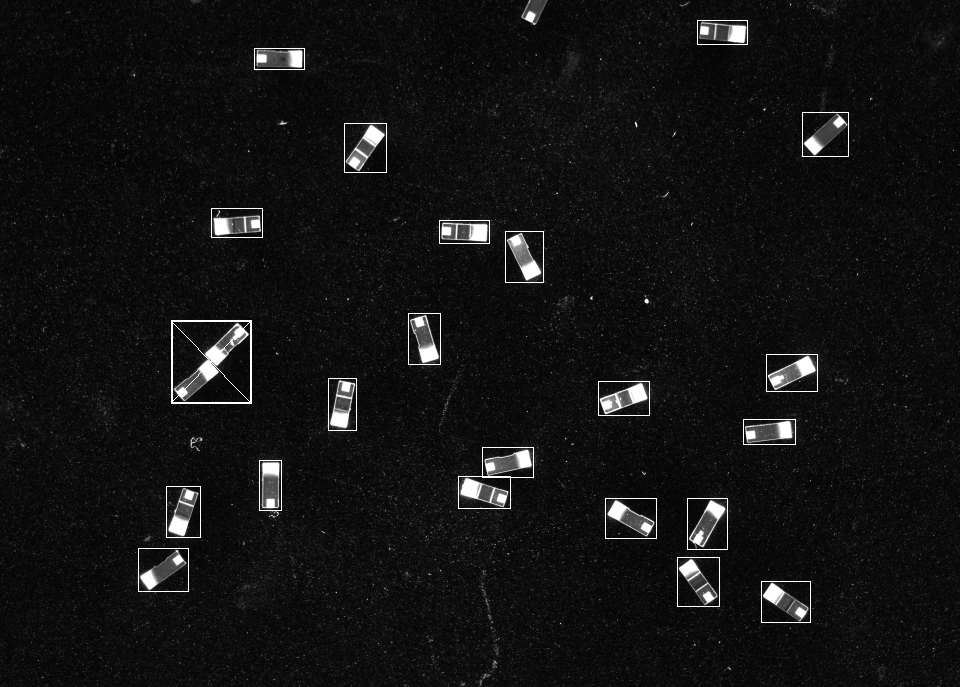
Figure 23.3 paints the results back onto the original image: good singles get thin white boxes, and the anomalous touching pair gets a thick white box with a diagonal cross. Reading this figure carefully reveals three things: the scattered felt specks have no box at all — the work of the area filter; the component clipped at the bottom edge is likewise unboxed — ignoreROIBoundary discarded it before classification; and that crossed thick box at the middle left is the single anomaly among the 21 good components — a pair of components touching end-to-end, and the protagonist of the next section.
23.4 Touching and Merging
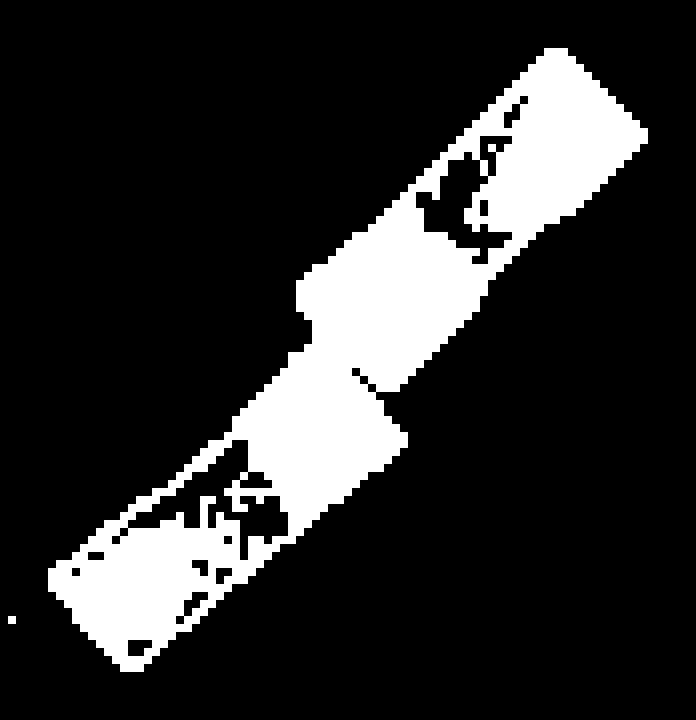
That touching pair is a nail already planted in the real sample: two chip components overlap end-to-end, their metallized faces connected at the seam, and after binarization they inevitably merge into one blob. Figure 23.4 (a) shows that area of the binary image magnified 8×: a “bent bar” with a narrow waist in the middle. Connected component labeling is helpless here; what it sees is one object.
The merged blob’s features expose the failure mechanism completely — and hand us the key to detecting it: area 1342 px (the median area of a good single component is 637 px, a ratio of 2.1) and anisometry 5.26 (a single is about 2.8, a ratio of nearly 2). Two pose-invariant criteria raise the alarm at once — which is exactly why it was classified as a reject in the previous section. Recovering the count, meanwhile, has a path lighter than morphology: the area quotient. Divide the merged blob’s area by the nominal single-component area, \(1342 / 637 = 2.11\), round to 2 — and this pair is restored in full. The component count for the whole frame is then \(21\ (\text{good}) + 2\ (\text{area-quotient recovery}) = \mathbf{23}\) (plus the one clipped by the bottom edge, left for the next frame).
Touching is not the fault of the connectivity choice — it is an inevitability of feeding: when parts are shaken loose onto the tray, some will always land end-to-end. Worth stressing is the contrast with the diagonal contact of the first section: these two components have genuinely overlapping pixel sets, so they merge under both 4- and 8-connectivity; switching connectivity cannot save you here — you can only detect it at the feature level, or break it up at the mechanical level by re-feeding.
The other classic countermeasure is separation by erosion (for the principle of erosion see Chapter 8): the merge usually happens at a narrow “neck,” and a few erosions should pinch it off. The experiment does exactly that — and teaches a lesson about real structured parts. These chips are not solid bright blocks but structured parts of “two bright end-faces + a dimmer body”; a single 3×3 erosion, while pinching off the touching neck, simultaneously severs each single component’s end-face from its body. Figure 23.4 (b) is the same area after one erosion: the bent bar did not split cleanly into two — it crumbled into several pieces. And the price lands on the table immediately: the count of component-sized blobs across the whole image jumps from 22 to 32 — erosion corrupts the count rather than fixing it.
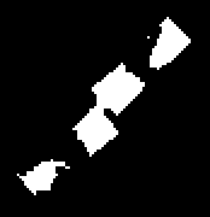
The engineering conclusion must be stated bluntly: on real structured parts, separation by erosion cannot be applied blindly. In a synthetic scene tangent circles are solid disks, and erosion merely shaves boundaries and splits them cleanly; but the moment a target has internal light/dark structure (metallized face vs body, plating vs base), erosion tears the good part open along its internal “dark seam,” distorting count and area together. The robust route on a real line is therefore to walk on two legs: detect the merge with pose-invariant features like area and anisometry (flag it as a reject and raise an alarm), and recover the count with the area quotient rather than the connected-component count. If you genuinely must cut the merge apart at the pixel level, watershed segmentation on the distance transform is far safer than blind erosion — it cuts along the “ridge” of the distance map without shaving off area, at the cost of a much heavier implementation and tuning.
23.5 SciVision Implementation
This chapter’s pipeline is the collaboration of three classes: SciSvThreshold produces the region, SciSvBlobAnalysis splits and filters, and SciSvRegionFeature computes the feature table.
// 1) Bright threshold: keep bright components in [80,255]; dstRegion and binary out together
SCIMV::SciSvThreshold th;
SciImage binImg;  SciRegion fgRegion;
th.ManualThreshold(img, roi, /*lower*/80, /*upper*/255,
                   SCI_THRESHOLD_TYPE_WHITE, 0, &binImg, &fgRegion);

// 2) Blob extraction: filter specks by area at extraction time + discard border-touching objects
SCIMV::SciSvBlobAnalysis ba;
SciRegion mask;                          // default-constructed = mask nothing
SciVarArray minV, maxV, ft;              // the triple for feature-interval filtering
ft.Append(SciVar((int)SCI_REGION_AREA));
minV.Append(SciVar(150.0));  maxV.Append(SciVar(5000.0));
SciVarArray fhF, fhMin, fhMax;           // left empty = no hole filling
SciRegionArray blobs;  SciMatrix featM;
ba.BlobAnalysis(fgRegion, img, roi, mask, minV, maxV, ft,
                /*fillHole=*/false, fhF, fhMin, fhMax,
                /*ignoreROIBoundary=*/true, false, &blobs, &featM);

// 2') Alternatively, extract wide open first, then post-filter by area with BlobFilter
ba.BlobFilter(blobsAll, featAll, SCI_REGION_AREA, 150.0, 5000.0,
              &featArea, &blobsArea);

// 3) Compute features over the blob array (area, centroid, bbox, anisometry, rectangularity...)
SCIMV::SciSvRegionFeature rf;
SciVarArray feats;                       // Append the SciFeatureType codes in order
SciMatrix m;
rf.CalRegionFeature(blobs, feats, &m);
Several parameters deserve individual comment. ManualThreshold takes the gray band [80,255], and SCI_THRESHOLD_TYPE_WHITE means “in-band is foreground” — just right for bright targets on a dark background; its last parameter dstRegion is an engineering treat: the segmentation result, as a SciRegion, feeds directly into the first parameter of BlobAnalysis, with no detour through a binary image and re-extraction. The three arrays minValue/maxValue/featureType of BlobAnalysis constitute the feature-interval filter applied at extraction time (this example sets only an area floor to strip specks); ignoreROIBoundary = true is the border-discard described in Section 23.3. BlobFilter provides after-the-fact filtering instead — grab the full set wide open first, then tighten as needed, which makes it easy during tuning to see exactly whom each gate filtered out (the numbers 479 → 23 → 22 were printed exactly this way). Note the full-image ROI uses GenRect1((0,0),(W,H)): the lower-right corner is exclusive, so passing \((W,H)\) covers the whole image, whereas \((W{-}1,H{-}1)\) would miss the outermost row and column.
Three pitfalls need to go on record. First, the row/column orientation of the SciMatrix output by CalRegionFeature is not documented — this chapter’s companion code auto-detects the orientation by checking which dimension’s length equals the number of features before reading values, and you must keep this layer of defense when porting. Second, the rectangularity SCI_REGION_RECTANGLEDEGREES is computed against the axis-aligned bounding rectangle and varies with the target’s angle (measured 0.38–0.93 across same-model components) — it cannot serve as a pose-invariant criterion; for a pose-invariant shape criterion use anisometry. Third, several headers including SciSvBlobAnalysis unconditionally define DLL_EXPORTS (i.e., they declare with dllexport); placing their #include after the dllimport-style headers links fine — verified in practice with no ill effect.
Industry Case: Rework for Touching Parts in Bulk Feeding
An SMD incoming-inspection line used a vibratory bowl to shake chip components onto an inspection tray, then ran blob analysis to count each tray and verify the specification. When the density rose, occasionally two components landed touching end-to-end, merged into one blob after binarization, and the count came up short by 1 — whereupon the system falsely alarmed “missing part” and stopped the line, even though not a single part was missing. Investigation found that every false-alarm frame contained one “big blob” with roughly twice the area of a normal component and nearly twice the anisometry — the touching pair. The line first tried to cut it apart with erosion, only to find these “end-face + body” structured parts crumbled under erosion and made the count worse. The final fix used no morphology but walked on two legs: a dual threshold on area and anisometry flagged the touching pair as anomalous and triggered the bowl to re-shake the tray (resolving the merge mechanically), while the “missing-part” criterion was changed from connected-component count to total foreground area divided by the nominal single-part area, rounded — the touching pair’s area quotient is \(1342/637\approx2\), recovering exactly the missing part. After deployment the false alarms dropped to zero. The lesson: in counting tasks, the “area quotient” is more robust than the “connected-component count” — merging changes the topology but barely changes the area; and on real structured parts, separation by erosion must be used with great caution.
23.6 Summary
- Blob analysis = connected components + features + filtering — the standard three-act play that turns a “heap of white pixels” into “countable objects”; the connectivity choice (4/8) decides whether diagonal contact counts as one or two, but a physical overlap merges the pixel sets and no connectivity choice can save it.
- Three principles of feature selection: interpretable, sensitive to target differences, insensitive to noise and pose. Area and anisometry are the most robust first-line features (this chapter’s singles hold anisometry at 2.7–3.4, the touching pair shoots to 5.26); axis-aligned rectangularity and bounding-box dimensions drift with rotation, and perimeter-based circularity is unreliable for small targets.
- Filtering is the prerequisite for classification: the area floor removes the felt specks, and
ignoreROIBoundarydiscards border objects that are truncated by the field of view and carry untrustworthy features — each step of this chapter’s 479 → 23 → 22 does its own job. - Touching is an inevitability of feeding, and separation by erosion depends on the target: synthetic solid targets split cleanly under erosion, but real “end-face + body” structured parts crumble (whole-image blobs 22→32), the count corrupted rather than fixed. The robust practice is to detect the merge with area/anisometry and recover the count with the area quotient, or switch to watershed; at the mechanical level, re-feed the tray.
- Blob features look only at the pixels’ “occupancy,” not at the boundary’s “shape trajectory” — when classification needs finer contour information, proceed to contour analysis (Chapter 24).
The algorithmic roots of connected component labeling trace back to Rosenfeld and Pfaltz’s foundational paper on sequential operations in digital pictures (Rosenfeld and Pfaltz 1966) — connected component labeling, the distance transform, and an early form of the skeleton all appear there; for the topological analysis and run-style extraction of region boundaries, see Suzuki and Abe’s border-following algorithm (Suzuki and Abe 1985). A textbook survey of connected component labeling and region features is given by Gonzalez and Woods (Gonzalez and Woods 2018); for a more systematic engineering treatment of region features and morphological segmentation (including watershed), see the book by Steger et al. (Steger, Ulrich, and Wiedemann 2018).