25 Shape Features
After the past several chapters, we already hold quite a few tools that “turn images into numbers”: blob analysis gives area and centroid (Chapter 23), contour analysis gives perimeter and circularity, edge detection gives position and direction. But the problems on a production line go far beyond these. For a meandering PCB trace, how should its “length” and “width” be defined? Two surfaces with exactly the same average brightness — one a uniform, acceptable coating, the other a reject covered in pits — what number tells them apart? When a board needs coarse localization, where do we find a few reference points that are “both sparse and stable”? This chapter gathers three tools — each independent, yet all answering “how to compress a shape into decidable numbers” — into one toolbox: the skeleton extracts the medial axis of elongated structures, gray-level and texture features extract a statistical fingerprint of surface appearance, and corners extract landmarks from geometric outlines. Figure 25.1 is the test scene for the skeleton experiments — a Y-shaped branching trace, an L-shaped trace, and a blob with a square hole, all typical samples that are 5 pixels wide or contain elongated/blocky structures.

25.1 Skeleton
Imagine placing the largest possible circle inside a binary shape and letting it roll around while always staying tangent to the boundary — the locus of all these maximal inscribed circle centers is the shape’s medial axis; attach to each center the radius of its inscribed circle and you obtain the medial axis transform. Intuitively, the medial axis is the shape’s “backbone”: for a trace of constant width, the medial axis is exactly the centerline along the trace direction, and the inscribed-circle radius is exactly the half-width. This is the most natural description of an elongated structure — it reduces a two-dimensional “patch of pixels” back to a one-dimensional “line plus a width.”
The medial axis is very sensitive to boundary noise: a small bump on the boundary makes the medial axis sprout an extra branch. Engineering implementations (including thinning algorithms) usually smooth the boundary first with the opening and closing operations of Chapter 8, or prune short branches (pruning).
In practice the most common way to compute a skeleton is a thinning algorithm: iteratively peel pixels off the shape’s boundary, while guaranteeing that no deletion ever changes connectivity — neither peeling one shape into two pieces nor peeling a hole out of existence — until only a single-pixel-wide centerline remains. It belongs to the family of morphological algorithms introduced in Chapter 8, and its output is a discrete approximation of the medial axis.
Running SciVision’s skeleton algorithm on Figure 25.1 gives the result in Figure 25.2. The three shapes produce 3 skeleton contours; the foreground of the entire scene contains 17729 pixels, while the skeleton retains only 738 — a 24.0-fold compression — and yet none of the topology or course information of the elongated structures is lost. Note the skeleton of the holed blob at the top right: it forms a closed loop around the square hole, which is precisely the “topology-preserving” property of thinning at work — the shape has one hole, so the skeleton has one loop that can neither be broken nor shrunk away.
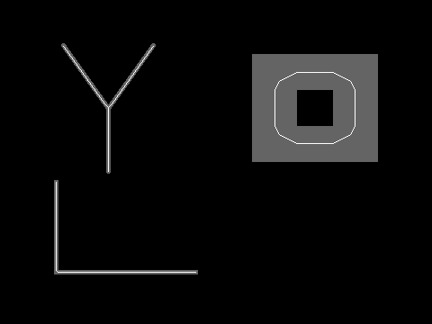
A skeleton is a structured curve, and the feature points on it carry engineering meaning of their own: an endpoint is where a trace starts or stops, and a junction is where it branches. Extracting feature points from the Y-shaped trace’s skeleton yields 3 endpoints and 1 junction, in exact agreement with ground truth; the endpoints lie at (70, 51), (120, 190), (170, 51), and the junction lies at (120, 119), just 1 pixel from the geometric ground truth of (120, 120). For trace inspection these two kinds of points are the “circuit diagram”: a wrong endpoint count means an open circuit, and a wrong junction count means a bridge.
The most important application pattern of the skeleton is a simple division:
\[ \bar{w} = \frac{A}{L}, \]
where \(A\) is the foreground area of the trace, \(L\) is the skeleton length (pixel count), and \(\bar{w}\) is the trace’s average width. Measured on the L-shaped trace in the scene (designed width exactly 5.00 px): area 1313 px, skeleton length 257 px, average width \(1313/257 = 5.11\) px. Where does the error come from? Skeleton length is counted as 4-connected pixels, and at the corner of the L the discrete count comes out slightly shorter than the geometric arc length (the corner gets “shortcut”); a smaller denominator naturally pushes the width slightly up. A 2% systematic bias is entirely adequate for trend monitoring, but for absolute pass/fail width judgments you should calibrate with arc length (counting diagonal steps as \(\sqrt{2}\)) or with caliper measurement. Honestly reporting this kind of discretization bias has more engineering value than pretending “measured = true.”
The skeleton’s typical uses can be listed in one inventory:
- Line-width inspection: area / skeleton length gives the average width; sampling the inscribed-circle radius point by point along the skeleton gives a width sequence;
- Open-circuit and bridge detection: count endpoints and junctions and compare against the design netlist;
- Path planning and length measurement: the “true length” of a meandering trace, a crack, or a fiber is its skeleton length.
25.2 Gray-Level and Texture Features
The question the second group of tools answers is: how does the surface appearance of a region become numbers? The first thing that comes to mind is first-order statistics — compute the gray-level histogram of all pixels in the region and take the mean, standard deviation, and entropy. They are cheap and intuitive, but they have one fundamental blind spot: first-order statistics see only “which gray values are present,” and are completely blind to “how those gray values are arranged.”
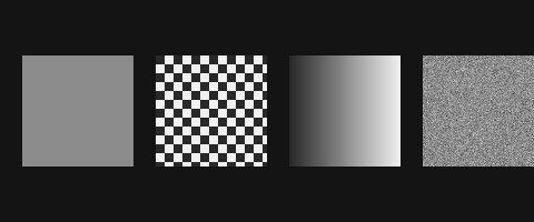
The four 100×100 texture regions in Figure 25.3 were designed precisely to expose this blind spot: uniform gray 140, a high-contrast checkerboard (alternating 40/240), a horizontal gradient (40→240), and Gaussian noise (\(\mu=140\), \(\sigma=20\)) — the means of all four regions are approximately 140 (measured 140.00 / 139.84 / 139.51 / 139.76). By the mean, the four regions are one and the same. The standard deviation opens up some gaps (0 / 100.00 / 58.18 / 20.04), but look at the entropy: 6.64 for the gradient region, 6.36 for the noise region — nearly identical. In the eyes of first-order statistics, a “smoothly transitioning gradient” and “scrambled noise” are hard to tell apart, because both spread their histograms wide.
To see “arrangement,” look at pixel pairs. The gray-level co-occurrence matrix (GLCM) counts, for a given direction and distance (most commonly: horizontally adjacent), the frequency \(P(i,j)\) with which a pixel of gray level \(i\) has a neighbor of gray level \(j\) — it is the joint distribution of the gray levels of adjacent pixel pairs. After quantizing the gray values into a small number of levels (16 in this experiment), the matrix is not large, yet the texture’s “arrangement law” is written entirely inside it: a uniform texture concentrates its energy in a single cell on the diagonal, a gradient texture concentrates in a narrow band near the diagonal, and a noise texture spreads across the whole matrix. From \(P(i,j)\) four common scalars are distilled:
- Energy \(\sum_{i,j} P(i,j)^2\): the more concentrated the distribution (the more uniform and regular the texture), the larger the value; 1 for a uniform region;
- Contrast \(\sum_{i,j} (i-j)^2 P(i,j)\): the larger the gray difference between adjacent pixels, the larger the value — a measure of “local contrast”;
- Correlation: the statistical correlation coefficient between \(i\) and \(j\) — the degree to which adjacent pixels “know each other”;
- Homogeneity \(\sum_{i,j} \frac{P(i,j)}{1+|i-j|}\): the closer the mass lies to the diagonal, the larger the value — a measure of “local smoothness.”
The GLCM has a direction: this experiment counts horizontally adjacent pairs. For isotropic textures (noise, uniform), the direction does not matter; for anisotropic textures (scratches, brushed finishes, the horizontal gradient in this example), switching direction changes the numbers completely — counting the gradient region in the vertical direction would yield a contrast of 0. In practice, either choose the direction from the known orientation of the defect, or average over the four directions.
The full measured table for the four regions is below (mean/standard deviation computed ourselves, for the reason given in Section 25.4; GLCM taken in the horizontal direction with 16 gray levels):
| Region | Mean | Std. dev. | Entropy (1st-order) | GLCM energy | Contrast | Correlation | Homogeneity |
|---|---|---|---|---|---|---|---|
| Uniform 140 | 140.00 | 0.00 | 0.00 | 1.000 | 0.000 | 0.000 | 1.000 |
| Checkerboard | 139.84 | 100.00 | 1.00 | 0.393 | 20.485 | 0.758 | 0.879 |
| Gradient | 139.51 | 58.18 | 6.64 | 0.061 | 0.131 | 0.996 | 0.934 |
| Noise \(\sigma=20\) | 139.76 | 20.04 | 6.36 | 0.048 | 3.350 | −0.015 | 0.467 |
Read the table row by row and ask “why this signature.” The uniform region is the degenerate case: only one gray level, so energy 1, homogeneity 1, contrast 0, and correlation undefined because the variance is zero (the SDK returns 0). The checkerboard region’s signature is high contrast (20.48, two orders of magnitude above the lowest non-trivial entry in the table): with 8 px squares, about 1/8 of the horizontally adjacent pairs straddle a black–white boundary, and every crossing contributes an enormous \((i-j)^2\); the remaining 7/8 of the pairs share a square and a gray level, which is why the correlation still reaches 0.758 — “violent contrast, but arranged with regularity.” The gradient region’s signature is high correlation (0.996) paired with low contrast (0.131): horizontally adjacent pixels differ by only about 2 gray levels and are almost perfectly predictable from one another — “large change, but change with order.” The noise region’s signature is low homogeneity (0.467, the lowest in the table) plus zero correlation (−0.015): adjacent pixels are mutually independent — neither can predict the other. Four regions with identical means each occupy their own corner in the four GLCM quantities, cleanly separable — and that is the value of second-order statistics: they turn “arrangement” into numbers.
25.3 Corners
The third group of tools hunts for geometric landmarks. What makes a corner special can be understood through the “self-similarity” of a small window: shift the window a small step in any direction and see how much its content changes. In a flat region, no shift in any direction changes anything; on an edge, shifting along the edge changes nothing while shifting perpendicular to it changes a lot — only one direction is “sensitive”; but at a corner, a shift in any direction changes the content drastically — there are strong gradients along two independent directions. The Harris corner detector (Harris and Stephens 1988) turns this intuition into an eigenvalue criterion on the gradient structure matrix within the window: only when both eigenvalues are large is it a corner.
The experimental scene is an L-shaped hexagonal plate (6 right angles, 1 of them concave) plus a distractor — a rounded rectangle with corner radius 25 px, which has no sharp corners at all. Extracting corners with the Harris method at a filter ratio of 0.30 gives the result in Figure 25.4 (a): exactly 6 corners detected, in one-to-one correspondence with ground truth, each corner sitting 1.41 px from its geometric truth — a consistent \((\pm 1, \pm 1)\) bias. That the bias is so tidy is no coincidence: the Harris response peaks where the gradient structure is richest, and for a right angle evaluated over a 5×5 neighborhood (blockSize=5), that peak lands stably one diagonal pixel from the corner. A systematic bias can be calibrated and compensated; random jitter is the true killer of accuracy — and this 1.41 px belongs to the former.

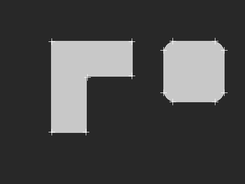
Lowering the filter ratio from 0.30 to 0.02 makes the detection count explode from 6 to 14 (Figure 25.4 (b)), 8 of which land on the four rounded corners of the rounded rectangle — each rounded corner detected as 2 “corners.” This reveals a fact that is often overlooked: corner “strength” is a continuous quantity; “whether it is a corner” is an engineering definition. At a rounded corner the curvature is nonzero, there really are gradients in both directions, and the Harris response really is greater than zero — just weaker than at a right angle. Wherever you set the threshold, that is where the boundary of “corner” lies. This is the same philosophy as the threshold tuning of Chapter 13: the algorithm outputs a response map, and the “decision” is always made by a human on the algorithm’s behalf. The tuning method is the same too — scan the threshold on samples containing known distractors and find the safe interval of “all true corners detected, zero rounded corners detected.”
What do you do once the corners are found? Three typical uses: use 2–3 stable corners for coarse localization of a workpiece (much faster than template matching); the grid intersections of a calibration plate are corners in essence, the input to camera calibration; and as interest points for feature matching — the first internal step of the feature matching in Chapter 18 is exactly the detection of these “changes no matter which way you shift” points.
25.4 SciVision Implementation
The skeleton is provided by SCIMV::SciSvSkeleton, with two interfaces used together:
SCIMV::SciSvSkeleton sk;
SciContourArray arr;
sk.Skeleton(src, roi, &arr);          // thinning -> array of skeleton contours
SciPointArray ends, juncs;
sk.ExtractJunctions(arr[i], &ends, &juncs);  // endpoints/junctions of a single contour
Skeleton thins every connected shape inside the ROI into a skeleton and outputs a contour array — note that it does not split at junctions: the entire skeleton of the Y-shaped trace is one contour, not three branches. This is deliberate engineering design: whether to split, and where, is decided by ExtractJunctions — it takes a single skeleton contour and outputs an endpoint array and a junction array, and the caller then splits at the junctions as needed. The two-stage “thinning is thinning, parsing is parsing” arrangement lets one API serve both the user who only wants a length and the user who wants the full topology.
Gray-level features are provided by SCIMV::SciSvGreyFeature:
SCIMV::SciSvGreyFeature gf;
double ent, aniso;
gf.GetEntropyGreyFeature(src, roi, &ent, &aniso);   // first-order entropy + anisotropy
double ge, en, corr, homog, contr;
gf.GetGLCMFeature(src, roi,
    SCI_SV_GREYFEATURE_GLCM_DIRECTION_HORIZONTAL,    // direction: horizontally adjacent pairs
    16,                                              // number of gray quantization levels
&ge, &en, &corr, &homog, &contr); // GLCM entropy/energy/correlation/homogeneity/contrastGetGLCMFeature’s greyClass=16 is the quantization level count: more levels mean a larger matrix and more sensitivity to noise; 16 is the common compromise. For the meaning of the direction parameter, see the margin note in Section 25.2. One reminder about an old pitfall: the stdValue of SciSvHistogram::CaculateHist is the standard deviation of the histogram bin counts, not the gray-level standard deviation, so the means and standard deviations in this chapter’s table were computed from the definition ourselves.
Corners are provided by SCIMV::SciSvCornerExtraction:
SCIMV::SciSvCornerExtraction ce;
SciPointArray pts;
ce.ExtractCorners(src, roi,
    0,        // method: 0 = Harris
    5,        // blockSize: evaluation neighborhood of the gradient structure matrix
    50,       // maxnumCorners: upper bound on count
    0.30,     // filterRatio: response filter ratio (the protagonist of this chapter's sensitivity experiment)
    10,       // minDistance: minimum distance between corners, suppresses duplicate detections of one corner
    &pts);
minDistance=10 explains why each rounded corner yields “only” 2 detections under the weak threshold — without it, detections would pop up along the entire arc. The complete project that generates all of this chapter’s images and data is located at code/shape_features/.
Industry Case: Open-Circuit Detection on Flexible PCBs
An FPC (flexible printed circuit) production line inspects trace health after etching. The initial scheme used blob connectivity analysis: a trace broken into two blobs was reported as an open circuit. It could only catch “fully broken,” while the necking caused by over-etching (a trace locally thinned but not yet severed) was missed entirely — and the necked parts failed in batches during bend testing. The improved scheme introduced the skeleton: extract the skeleton of each trace and compute, in a sliding window along the skeleton, “local area / local skeleton length,” yielding a width sequence along the trace. The width sequence of a healthy trace is flat; a neck appears as a clear valley in the sequence — set a lower width limit, and a half-broken trace is intercepted before it breaks. The lesson: the skeleton reduces “two-dimensional shape health” to a “one-dimensional signal,” and on a one-dimensional signal the classic threshold, trend, and SPC tools all become immediately applicable — dimensionality reduction is not losing information; it is placing the information within reach of the old tools.
25.5 Summary
- The skeleton is the medial axis of elongated structures: thinning iteratively peels the boundary while preserving topology (holes become closed loops), compressing a 17729 px foreground into a 738 px centerline (24-fold) without losing course or topology; endpoints/junctions map directly to open-circuit/bridge criteria.
- Width = area / skeleton length is the skeleton’s most practical pattern (measured 5.11 vs ground truth 5.00); pixel counting underestimates arc length at corners, introducing about a 2% systematic bias — negligible for trend monitoring, but absolute judgments require calibration.
- First-order statistics cannot see “arrangement”: four texture regions all with mean 140 cannot be fully distinguished by mean and entropy; the GLCM turns the joint distribution of adjacent pixel pairs into the four numbers energy/contrast/correlation/homogeneity, giving each region a unique signature (checkerboard = high contrast, gradient = high correlation with low contrast, noise = low homogeneity with zero correlation).
- Corner strength is a continuous quantity; “whether it is a corner” is an engineering definition: filterRatio=0.30 detects exactly 6 corners with a consistent 1.41 px bias (calibratable); loosening to 0.02 lets the rounded-corner distractor contribute 8 false detections — threshold tuning must scan samples that contain distractors.
- What the three tools share is compression: squeezing a patch of pixels into a line, a distribution, or a few points is what gives downstream decision logic something to hold on to.
The original definition of the medial axis comes from Blum’s shape-description transform (Blum 1967), the theoretical parent of this chapter’s skeleton; the canonical source of GLCM texture features is Haralick et al.’s foundational paper on texture-based image classification (Haralick, Shanmugam, and Dinstein 1973); the Shi–Tomasi corner criterion (Shi and Tomasi 1994), a sibling of the Harris corner (Harris and Stephens 1988) and widely used for coarse workpiece localization, is given there; and for pose-invariant shape descriptors, Hu’s moment invariants (Hu 1962) remain an enduring classic. For the rigorous definitions of the skeleton and the medial axis transform, and a systematic engineering discussion of GLCM texture features, see the book by Steger et al. (Steger, Ulrich, and Wiedemann 2018).