29 Classical Classifiers
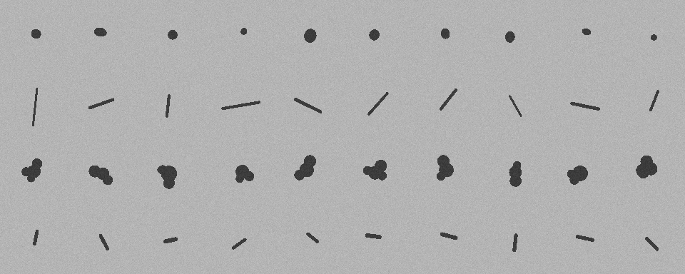
Throughout the recognition part of this book we have, in fact, been doing classification all along — only in increasingly free forms. Barcode recognition is essentially “table lookup”: the symbology pre-encodes the answer into black-and-white bars and spaces, and the algorithm merely decodes; OCR widens the scope to a few dozen character classes, but the character set is known and closed. This chapter faces the general classification problem itself: given a target, decide which of the predefined classes it belongs to — is that blemish on a tablet a black dot, a fiber, or a clump of debris? Problems like this have no encoding rules to lean on; statistical regularities can only be learned from samples. Before deep learning swept through the vision field, k-nearest neighbors (KNN), the multilayer perceptron (MLP), and the support vector machine (SVM) were the “big three” of pattern recognition; to this day, in industrial tasks with low feature dimensionality, small sample sizes, and a need for interpretability, they remain the kings of cost-effectiveness — training takes seconds, prediction takes microseconds, no GPU is required, and when a misclassification occurs you can trace the cause. This chapter threads a foreign-object sorting task through all three classifiers: distinguishing three kinds of dark targets on a bright background — round dots, elongated fibers, and irregular clusters — as shown in the first three rows of Figure 29.1; the “fat capsules” in the fourth row are deliberately manufactured borderline samples, which we save for making trouble later.
29.1 Feature Space and Separability
Classifiers do not consume images directly. The first step is to turn each image into a feature vector: after threshold segmentation yields the target region, the region features introduced in Chapter 23 compress it into 4 numbers — area, anisometry, circularity, and compactness. Each sample thus becomes a point in a four-dimensional feature space, and “classification” becomes the geometric problem of carving up territory in this space.
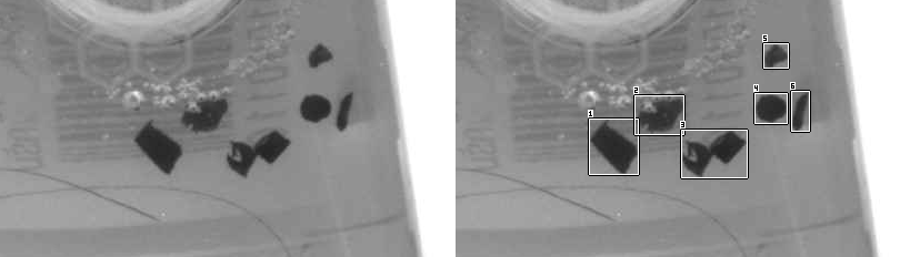
What does real production foreign matter look like? Figure 29.2 is taken from one frame of the OPT Smart3 deep-learning sample project — a translucent cosmetic tube with several dark foreign particles scattered across its surface. We process it through exactly the same pipeline as above: place an ROI over the particle cluster, threshold-segment (the tube body is bright, the particles near-black), use blob analysis to filter out the printed halftone dots, and then extract the same 4-D region features for each particle. The 6 segmented particles and their real measured values are:
| Particle | area | aniso | circ | comp | morphology |
|---|---|---|---|---|---|
| P1 | 1143 | 1.67 | 0.500 | 1.40 | blocky chip (cluster-like) |
| P2 | 902 | 1.64 | 0.478 | 2.14 | blocky chip (cluster-like) |
| P3 | 1180 | 2.29 | 0.358 | 2.21 | blocky chip (cluster-like) |
| P4 | 562 | 1.14 | 0.753 | 1.09 | compact dark spot (dot-like) |
| P5 | 294 | 1.33 | 0.571 | 1.20 | compact dark spot (dot-like) |
| P6 | 322 | 3.28 | 0.280 | 1.73 | elongated sliver (fiber-like) |
These real measurements confirm that the synthetic task setup is not invented out of thin air: P4 and P5 are compact dark spots (circularity 0.57–0.75, anisometry near 1), corresponding to “dots”; P1–P3 are larger blocky chips with broken edges (circularity 0.36–0.50), corresponding to “clusters”; P6 is an elongated sliver (anisometry 3.28, circularity only 0.28), leaning toward “fiber.” Real foreign matter does spread along the same dot–fiber–cluster morphology continuum, so the feature design of this chapter rests on real ground.
But precisely because it is “real,” the classifier training and evaluation cannot rest on it, for three reasons. First, a single frame holds only 6 particles and carries no per-particle ground-truth class labels, so there is no way to assemble a 40/20 train/test split per class. Second, the morphology spectrum of real foreign matter is continuous — P6’s anisometry of 3.28 sits right at the lower edge of the “fat capsule” borderline interval (3.33–5.16) we synthesize later, leaving no clean gap between classes to compare the three classifiers’ boundary behavior fairly. Third, a controlled synthetic set lets us dial separability, sample size, and boundary difficulty precisely — exactly the “test bench” the experiments below require. The division of labor in this chapter is therefore: the real sample image verifies that feature extraction and the morphology spectrum are genuine, while classifier training and the comparative experiments run on a controlled synthetic set that is labelable, splittable, and difficulty-adjustable (the synthetic samples are shown in Figure 29.1).
Figure 29.3 projects this controlled synthetic dataset onto the anisometry × circularity plane. The layout of the three classes is plain at a glance: the fibers (crosses) hang alone in the lower right — anisometry 7.15–18.0, circularity a mere 0.07–0.15, neighbors to no one; the dots (filled disks) and clusters (hollow squares), by contrast, crowd together in the upper left — the dots’ anisometry range of 1.00–1.48 almost coincides with the clusters’ 1.09–2.17, and their circularity intervals (0.50–0.79 versus 0.41–0.68) overlap over a wide stretch. On these two dimensions alone, no classifier whatsoever could pull them apart. The rescue comes from the other two dimensions: dot area runs 54–340, cluster area 373–807 — one clean cut; compactness (0.90–1.09 versus 1.17–1.66) is just as cleanly divided. The gray diamonds are those 10 borderline capsules, with anisometry 3.33–5.16, perched squarely in the vacuum zone between dots and fibers.
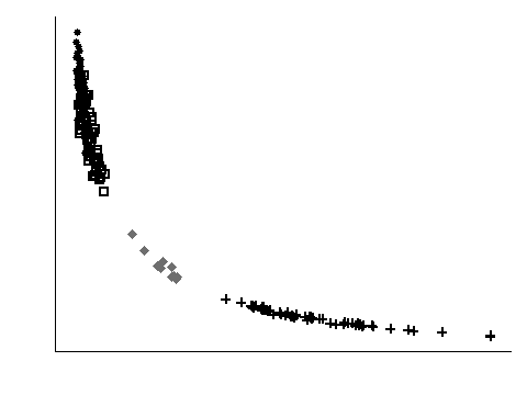
This figure delivers the first — and possibly the most important — conclusion of this chapter: separability depends first on feature selection, and only then on the classifier. With the right features, the three classes sit far apart in four-dimensional space and even the plainest classifier gets everything right; with the wrong features — say, only the first two dimensions — the most ingenious model has nothing to work with. When troubleshooting poor classification results in engineering practice, you should first plot the feature scatter and check separability, rather than rushing to swap models and tune parameters.
The division of labor between feature engineering and end-to-end learning: deep networks hand “feature extraction” over to learning as well, at the cost of needing large amounts of labeled data; classical classifiers hand the features to domain knowledge (shape, texture, color statistics), leaving learning responsible only for drawing boundaries in a low-dimensional space. Industrial tasks often have few samples but well-understood mechanisms — landing squarely in the latter’s comfort zone.
29.2 The Geometry of Three Classifiers
All three classifiers learn a mapping from vectors to classes in feature space, \(f:\mathbb{R}^4 \to \{\text{dot},\text{fiber},\text{cluster}\}\), but their “worldviews” could hardly differ more.
KNN does not learn; it memorizes. The training phase merely stores all the samples (in practice building a kd-tree to speed up retrieval); at prediction time it finds the \(K\) training samples nearest to the query point and lets them vote. Its decisions are entirely local: the boundary is determined by the positions of a handful of samples, and if the samples carry noise, the boundary turns mottled and jagged along with them. Its strengths spring from the same source — zero training cost, instant effect when samples are added or removed, and every verdict can point to “which neighbors cast the votes.” Since the features differ wildly in scale (area in the hundreds, circularity below 1), the data must be normalized before distance computation, or the area dimension alone will dominate the distance.
The MLP learns a smooth function. The input layer’s 4 nodes correspond to the features, the hidden layer applies a nonlinear transformation, and the output layer’s 3 nodes, after normalization, give a soft score for each class, with the maximum taken as the verdict. Training fits iteratively via backpropagation — it is the only one of the three that has to “learn slowly.” Its decisions are global: all training samples jointly shape one continuous surface, individual noisy samples get averaged away, and the boundary is therefore smooth. The price is randomness in training, a hidden-layer size that must be specified by hand, and the fact that the soft scores are merely a byproduct of curve fitting, not calibrated probabilities — a point illustrated with a concrete example later.
The SVM cares only about the vicinity of the boundary. It seeks the hyperplane that separates two classes with the maximum margin; the hyperplane is determined solely by the few support vectors hugging the margin — no matter how many samples sit farther away, they play no part. Combined with the kernel trick — this chapter uses the radial basis function (RBF) kernel — it can draw a linear boundary in an implicit high-dimensional space, which becomes a curved boundary back in the original space. The decision function takes the form
\[ f(\mathbf{x}) = \operatorname{sign}\Big(\sum_{i} \alpha_i y_i\, k(\mathbf{x}_i, \mathbf{x}) + b\Big), \]
where the sum runs only over the support vectors. Multiclass classification is assembled from multiple two-class decisions.
The choice of \(K\) is KNN’s only hyperparameter: \(K=1\) gives the most fragmented boundary and the highest noise sensitivity; as \(K\) grows the boundary smooths out, but small classes get “drowned” by large ones. This chapter uses \(K=3\) — enough for an actual vote (so a single noisy neighbor cannot decide alone), yet not so large as to flatten the local structure at a scale of 40 samples per class.
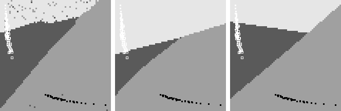
The three worldviews projected onto a plane become Figure 29.4. We fix area and compactness at their training-set means (301.5 and 2.15) and query the three trained models point by point over a 72×72 grid on the anisometry × circularity plane. KNN (left) shows a mottled upper half — the fixed area value happens to fall between dots and clusters, this region is close to neither class’s samples, the verdict flip-flops in a tug-of-war between neighbors, and isolated “enclaves” are scattered on the right; the MLP (center) produces a textbook-clean smooth boundary; the SVM’s boundary (right) is stitched from several nearly straight arcs — each one the meeting line of the RBF influence zones of a few support vectors. The three panels classify the same data with near-identical accuracy, yet the shapes of the boundaries faithfully expose each model’s inductive bias: local memory, global fitting, maximum margin.
29.3 Experiment: Accuracy versus Sample Size
The 60 samples per class are split 40/20 into training and test sets, and we then cut the training set down to 5 per class, and even 2 per class, to examine the effect of sample size. The full results follow (the test set stays fixed at 3×20):
| Classifier | Train 120 (40/class) | Train 15 (5/class) | Train 6 (2/class) |
|---|---|---|---|
| KNN (\(K=3\), z-score, kd-tree) | 100% | 98.3%1 | 100% |
| MLP (4-6-3, 500 iterations) | 100% | 100% | 100% |
| SVM (NU-SVC, RBF kernel) | 100% | 100% | 100% |
The honest conclusion is: nobody collapses. Even with only 2 training samples per class, all three classifiers remain almost perfect — because the three classes are far apart in feature space to begin with, and 2 points suffice to stake out each territory. This is the converse confirmation of the previous section’s claim: a task with good separability is insensitive to both classifier choice and sample size; the differences between classifiers only surface in borderline territory and on genuinely hard small-sample problems. Expecting an “easy” acceptance dataset to rank three classifiers against each other is a common methodological mistake in production-line model selection.
One entry in the table must be disclosed honestly: KNN’s accuracy is unstable across runs — the SDK’s kd-tree construction is nondeterministic, so rerunning on the very same data produces occasional flips in KNN’s verdicts — measured over 5 reruns the accuracy fluctuated between 91.7% and 100%, with up to 5 samples flipping in a single run, and the flips are not pinned to any particular training-size tier. The MLP and SVM results, by contrast, are fully reproducible.
29.4 The Ambiguous Zone: Three Semantics of Confidence
Now bring out those 10 fat capsules from the fourth row. Their anisometry of 3.33–5.16 falls in the no-man’s-land between dots (≤1.48) and fibers (≥7.15); there is no ground truth — what interests us is not “right or wrong” but how three classifiers trained on the same data will rule, and how each of them expresses “how sure it is.”
The result is a genuine three-way disagreement: KNN labels 8 as fiber and 2 as dot; the MLP labels all 10 as dot; the SVM labels 9 as fiber and 1 as cluster. Same training set, same query points, and three inductive biases deliver three answers: KNN looks locally — the capsules sit closer to the fiber sample cloud, so the neighbor vote tips toward fiber; the MLP’s globally smooth surface extrapolates the dots’ territory clear across the no-man’s-land; the SVM’s margin midline assigns most capsules to the fiber side, while the most circular one (anisometry 3.33) gets pushed to the third party — cluster. What classifiers’ disagreement at the boundary exposes is not who is right and who is wrong, but their respective inductive biases — wherever the training data offers no coverage, a model can only fill in the blanks according to its own worldview.
Of greater engineering value is how the three express confidence. KNN reports the neighbors’ votes and similarities: the 8 samples ruled fiber got unanimous 3-vote verdicts, while one sample ruled dot came out as “dot votes 0.667 (similarity 0.613), fiber votes 0.333 (similarity 0.635)” — the votes and the similarities even contradict each other; the hesitation is written all over its face. The MLP reports soft scores: nearly half the capsules receive a perfect dot=1.000, and most of the rest score above 0.95 (the lowest being 0.703) — a reminder, once again, that soft scores are a byproduct of surface extrapolation: a high score does not mean high reliability, and the farther from the training data, the more it must be discounted. The SVM in this SDK is the bluntest of all: it gives only a hard label — no score, no margin distance, not even a channel through which to express “hesitation.”
Rejection is a standard requirement of industrial classification: better to pull out doubtful samples for manual review than to let misclassifications escape. The prerequisite for rejection is that the classifier outputs comparable confidences that can be thresholded — the same mechanism as using minScore to cull low-scoring characters in Chapter 28.
This leads to an iron law of model selection: a production line that needs rejection or a manual-review safety net must choose a classifier with usable confidence output. This SDK’s SVM outputs hard labels, which means that on such a line it cannot support a “low confidence goes to a human” workflow — no matter how pretty its accuracy.
29.5 SciVision Implementation
The three classifiers are provided by SciSvKNNClassifier, SciSvMLPClassifier, and SciSvSVMClassifier, with an identical calling skeleton: initialize → AddSample per sample → Train → Classify.
// KNN: no training process; Train merely builds the index
SCIMV::SciSvKNNClassifier knn;
knn.InitializeModel(4, featNames);            // feature dimension + array of feature names
knn.AddSample(featVec, className);            // add samples one by one (4-dim SciVarArray + class name)
knn.Train(SCI_KNN_Z_SCORE, SCI_KNN_KDTREE);   // z-score normalization, kd-tree index
knn.Classify(3, SCI_KNN_MAX_COUNT, fv,        // K=3, majority vote
             &cls, &score, &names, &votes, &sims);  // outputs neighbor votes and similarities

// MLP: 4-6-3 fully connected network
SCIMV::SciSvMLPClassifier mlp;
mlp.LoadModel(path);                          // must be called first! a nonexistent file is fine (see below)
mlp.InitializeModel(0, 4, 6, 3);              // mode 0 = feature classification; input/hidden/output node counts
mlp.SetNames(featNames, classNames);
mlp.Train(500, 1e-6f, 0.0f, 1, 0);            // max iterations, error tolerance, no regularization, standardization
mlp.Classify(fv, &cls, &score, &names, &scores);    // outputs soft scores for all classes

// SVM: NU-SVC + RBF kernel
SCIMV::SciSvSVMClassifier svm;
svm.LoadModel(path);                          // likewise must be called first
svm.InitializeModel(featNames, 4, SCI_SVM_NU_SVC, 0.01, SCI_SVM_RBF, 1.0, 1.0, 0.0);
svm.Train(1000, 1e-6f, 1);                    // min-max standardization
svm.Classify(fv, &cls, &names);               // hard label only; no scores / margin output
The APIs themselves all run, but this group of modules harbors the most severe batch of SDK defects encountered in this book — multiple instances of cross-module, process-level state corruption, all pinned down through repeated experiments and recorded here verbatim:
- KNN
Trainreliably crashes (0xC0000005) afterManualThreshold: once threshold segmentation has been called anywhere in the same process, any subsequent KNN training hits an access violation. This forced this chapter’s example to be split into two process runs:demo.exe extracthandles data synthesis, threshold segmentation, and feature extraction, then writes outfeatures.csv;demo.exe classifystarts a fresh process that reads the CSV and performs training and evaluation. Handing off between feature extraction and classification via a plain text file is currently the only reliable isolation. - Training KNN after both the MLP and SVM have been trained yields a silently broken model: no error, no crash, but the cluster class tests 0/20 — every one wrong. The workaround is to organize the code as “KNN block → MLP block → SVM block,” finishing all of one classifier’s training and prediction before touching the next.
- After roughly 100 KNN
Classifycalls, the next KNNTrainin the same process crashes or produces a broken model (measured: 10 calls safe, 100 calls crash): within each block, all models must be trained first before batch prediction begins. - KNN
Trainwith treeType=1 (brute-force search) makes the subsequentClassifycrash — only the kd-tree (0) can be used; and the kd-tree in turn is nondeterministic across runs (the root of the ±1 flips in the previous section). LoadModelmust be called once before the MLP’s/SVM’sInitializeModel, otherwise error 122706011/122707003 — passing a nonexistent file path is fine; getting back the “new empty model created” code is enough to proceed.- Under KNN normalization modes 0/1, the class-name strings returned by
Classifyare occasionally garbled — with z-score (mode 2) the problem has not been observed.
The methodological significance of this list is no less than its content: a commercial library’s stability boundaries are not written in the manual — they can only be charted through systematic experiment — hold everything else fixed, introduce modules one at a time, and use probe programs to locate the crash thresholds, the same line of thinking as using golden experiments to reverse-engineer the true behavior of interfaces in Chapter 5. Write the workarounds, together with their full backstory, into the code comments (see the file header of code/classical_classifiers/main.cpp), so that those who come after need not step on the same mines.
Industry Case: The Feature Debate in Leather Texture Sorting
A synthetic-leather production line needed to sort finished product into three grades by texture coarseness. The first version of the solution scaled down the entire raw image and fed it straight to an MLP: the “end-to-end” accuracy barely cleared eighty percent, was extremely sensitive to illumination drift, and required retraining every time a lamp was changed. After a post-mortem, the project switched to the classical route: for each image, first compute four GLCM texture features — energy, contrast, correlation, and homogeneity (see Chapter 25) — then classify with KNN in this four-dimensional space. Accuracy overtook the original solution by more than ten percentage points and remained stable under illumination drift — texture statistics are naturally insensitive to overall brightness changes. Even more popular with the quality inspectors was the interpretability: for every misclassified sample, its 3 nearest-neighbor images could be pulled up for manual comparison, making it obvious at a glance “who” a borderline-grade leather surface resembled. The lesson: on small-data industrial tasks, good features + a simple classifier usually beats raw data + a complex model.
29.6 Summary
- Separability comes before the classifier: the success or failure of a classification problem is largely decided at the feature-selection stage. In this chapter’s task, dots and clusters overlap completely in the anisometry × circularity projection and are only separated by area and compactness — when troubleshooting a classification problem, plot the feature scatter first.
- Three inductive biases: KNN is local memory (mottled boundaries, verdicts traceable to neighbors), the MLP is a globally smooth function (soft scores, iterative training required), the SVM is maximum margin + kernel trick (the boundary determined solely by the support vectors). On easily separable tasks the three are hard to tell apart — even 2 training samples per class yield near-perfect accuracy; the differences only show in borderline territory.
- Confidence semantics differ across the board: neighbor votes + similarities, soft scores, hard labels — 10 borderline capsules made three classifiers, each 100% accurate, hand down three different rulings of 8:2, 10:0, and 9:1. A production line that needs rejection and manual review must choose a classifier whose confidence output is usable and thresholdable.
- A commercial library’s stability boundaries must be charted by experiment: this chapter’s SDK classifier modules suffer cross-module memory corruption, and the workarounds (feature extraction and classification in two separate processes; train everything first, then batch-predict) came from systematic crash-localization experiments, not from the manual.
- For a more systematic theory of classifiers (Bayesian decision theory, feature selection, and novelty detection), see the classification chapters of the book by Steger et al. (Steger, Ulrich, and Wiedemann 2018), together with two standard pattern-recognition textbooks (Duda, Hart, and Stork 2001; Bishop 2006). The founding paper behind each of this chapter’s three classifiers is worth returning to in the original: the asymptotic error bound of KNN is given by Cover and Hart (Cover and Hart 1967), the back-propagation that MLP training relies on was established by Rumelhart, Hinton, and Williams (Rumelhart, Hinton, and Williams 1986), and the SVM (with its maximum margin and kernel trick) originates in the support-vector networks of Cortes and Vapnik (Cortes and Vapnik 1995).
Here the recognition part of the book draws to a close. From the deterministic decoding of barcodes, to OCR’s closed-set character classification, to this chapter’s statistical decisions over an open feature space — three chapters have traversed the spectrum “from table lookup to learning”: what encoding rules can govern goes to the decoder, what rules cannot govern goes to features and classifiers, and the borderline territory that classifiers cannot govern is left to confidence measures and manual review.
A single representative run; measured over 5 reruns the accuracy ranged from 91.7% to 100%, and the nondeterminism is not confined to this training-size tier↩︎