16 Template Matching
“Where is this thing in the image?” — that is the question industrial vision gets asked most often: where on the tray is the part the robot arm must pick? By how much is the pad the placement head must align to offset? Where does the measurement program’s fiducial land in this frame? The most direct answer to this question is to take a “photo” of the target and compare it against the image position by position, looking for the spot that resembles it most. This is template matching: take a small reference image as the template, slide it across the search image comparing as you go, and output the position (and angle) of highest similarity. It needs no modeling, no training samples, and works on arbitrary texture — it is, deservedly, the workhorse of industrial localization.
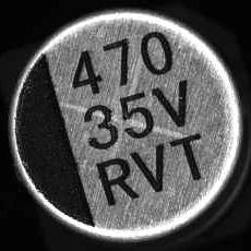
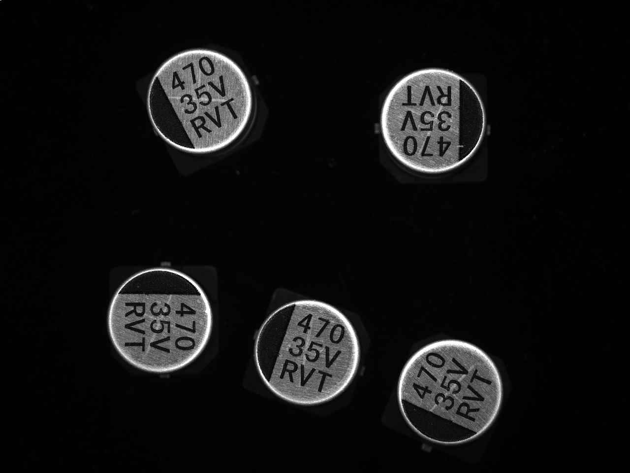
This chapter runs from start to finish on a set of real sample images: surface-mount aluminum electrolytic capacitors (rated 470 µF, 35 V, RVT series) scattered on a black background, provided by the Smart3 gray-value-matching example recipe (\(1280\times 960\) single-channel grayscale). Each capacitor is a reflective metal disc whose top face carries the silkscreen “470 / 35V / RVT” in three lines, with a dark polarity stripe on the left — stripe and text together break the circular rotational symmetry, giving the angle a unique solution. The template is cropped from one capacitor in the upper left of sample 001 (Figure 16.1 (a)): a \(230\times 230\) window around its disc top (disc diameter about 214 px). The search image is sample 003 (Figure 16.1 (b)), on which five capacitors of the same type are scattered at differing positions and poses: some upright, some rotated by small angles, and one flipped by nearly \(180^\circ\) — exactly how parts look after being fed onto a line. Section 16.5 further validates the same model on samples 004 and 005.
16.1 Similarity Measures
Align the top-left corner of the template \(t(u,v)\) with position \((x,y)\) of the search image \(f\); “how alike is it?” needs a number for an answer — this is a similarity measure. The two plainest are accumulations of pixel-wise differences: the sum of absolute differences (SAD) and the sum of squared differences (SSD):
\[ D_{\mathrm{SAD}}(x,y)=\sum_{u,v}\bigl|f(x{+}u,\,y{+}v)-t(u,v)\bigr|, \qquad D_{\mathrm{SSD}}(x,y)=\sum_{u,v}\bigl(f(x{+}u,\,y{+}v)-t(u,v)\bigr)^2 . \]
For both, smaller means more alike; they are cheap to compute and plain in meaning, but they carry one defect that is fatal on a production line: sensitivity to brightness changes. Suppose the window content somewhere happens to be the template multiplied by an illumination gain \(g\) (lights getting stronger or weaker, batch-to-batch differences in workpiece surface reflectance — all produce this kind of linear change); then
\[ D_{\mathrm{SSD}}=\sum_{u,v}\bigl(g\,t(u,v)-t(u,v)\bigr)^2=(g-1)^2\sum_{u,v}t(u,v)^2 . \]
The shape matches to the last detail, yet the residual grows quadratically with the gain deviation — let the lighting shift, and a “perfect match” looks “far off” in the eyes of SSD.
The remedy is to “standardize” the window and the template separately before comparing: subtract the mean (removing the brightness offset), divide by the standard deviation (removing the gain) — what remains is pure “shape.” This is normalized cross-correlation (NCC):
\[ \rho(x,y)=\frac{\displaystyle\sum_{u,v}\bigl(f(x{+}u,\,y{+}v)-\bar f_{x,y}\bigr)\bigl(t(u,v)-\bar t\,\bigr)} {\sqrt{\displaystyle\sum_{u,v}\bigl(f(x{+}u,\,y{+}v)-\bar f_{x,y}\bigr)^2}\;\sqrt{\displaystyle\sum_{u,v}\bigl(t(u,v)-\bar t\,\bigr)^2}}, \]
where \(\bar f_{x,y}\) is the mean of the current window and \(\bar t\) is the template mean. Its invariance to linear illumination changes can be seen through in one line: replace the window content by \(a f + b\) (with \(a>0\)); the mean subtraction eliminates the offset \(b\) in one step, and the gain \(a\), appearing as a common factor in numerator and denominator, cancels — \(\rho\) does not budge.
A geometric view: regard the mean-subtracted window and template each as a high-dimensional vector; NCC is then the cosine of the angle between the two vectors, hence always \(|\rho|\le 1\); \(\rho=1\) holds if and only if the window is a positive linear transform of the template, and \(\rho=-1\) corresponds to a black-white inversion (opposite polarity) — exactly the situation the SDK’s polarity parameter distinguishes.
The experiment confirms the derivation. Scanning sample 003 pixel by pixel with the fixed \(0^\circ\) template cropped from sample 001, the highest response lands on the nearly upright instance in the upper left, with an NCC of 0.827. That this does not reach close to 1 is precisely because the instance itself still carries about \(12^\circ\) of residual rotation relative to the template (see the angle-search result in Section 16.5) — a fixed-angle template cannot even align the “best” instance, a foreshadowing we defer to Section 16.3. To isolate NCC’s illumination invariance, we apply a controlled and openly disclosed perturbation to the real image: multiply the gray values within this instance’s neighbourhood wholesale by 0.5, emulating the illumination at this station dropping by half. The result is plain — NCC moves from 0.827 to 0.827 (a change of 0.0001), not budging; yet the root-mean-square SSD residual (rms) at the same position rises from 41.2 to 62.3, about a factor of 1.5. If a detection threshold with 40% margin is calibrated on the bright instance, the verdicts come out as follows:
| Measure and threshold | Bright instance | 50% illumination instance |
|---|---|---|
| SSD (rms \(\le 58\)) | detected (41.2) | missed (62.3) |
| NCC (\(\rho \ge 0.80\)) | detected (0.827) | detected (0.827) |
One utterly ordinary decay of the lighting is enough for SSD to declare a good part “absent.” NCC carries a further engineering benefit: its score naturally lies in \([-1,1]\) (the SDK converts it to a 0–100 scale), so a “pass score” threshold transfers directly across stations and cameras; an SSD threshold, by contrast, depends on the gray-value scale and the noise level — swap the camera and you must recalibrate. This is why industrial matching almost universally uses NCC (or the shape matching of the next chapter).
16.2 Score Maps and Peaks
Arrange the similarity at every position into an image and you obtain the score map. Figure 16.2 shows the NCC score map and the SSD score map of the same scene (the latter displayed as “bright = small residual”). To bring the cost of a full-resolution full-image scan down to a demonstrable range, both maps are computed at \(1/2\) resolution (\(640\times 480\)) with a \(115\times 115\) template (the reason is given in Section 16.4).
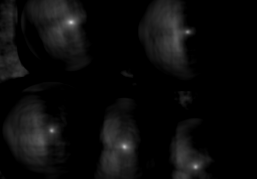
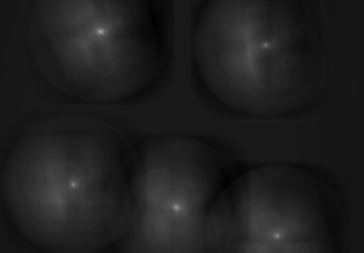
On the NCC score map each of the five capacitors raises a circular response, but the peaks are clearly graded: under the fixed \(0^\circ\) template the five instances’ peak values descend from 0.827 (upright) to 0.750, 0.656, 0.622, and 0.516 — the more an instance departs from the template pose, the lower the correlation, and the instance flipped by nearly \(180^\circ\) is left with only a faint response just over 0.5. This is precisely the lead-in to the next section: NCC is helpless against rotation. The SSD map tells the same story in its “residual” version: the upright instance is the brightest blob, and the brightness of the rest collapses fast.
The score map also reveals a deeper fact: the sharpness of a peak is the localization power. The sharper the peak, the faster the score falls off around the optimum, and the less room noise has to nudge the summit aside; conversely, a gentle ridge-like response means a string of positions are “about equally alike,” and localization is bound to wander. The richer the high-frequency structure in the template (disc edge, polarity stripe, silkscreen text), the sharper the peak. Finally, the integer-pixel summit is only the starting point: within the peak’s neighborhood, apply three-point parabola vertex interpolation to the scores along \(x\) and \(y\) separately (the \(\delta=(g_{-1}-g_{+1})/(2(g_{-1}-2g_0+g_{+1}))\) derived in Chapter 2) to refine the position to subpixel — fractional coordinates such as the \((404.07, 204.06)\) reported by commercial matchers come exactly from this.
16.3 Rotation and Pose Search
NCC solves illumination but is helpless against rotation: on sample 003 the fixed \(0^\circ\) template scores only 0.827 even on the best-aligned instance (which itself is still turned by about \(12^\circ\)), and the instance flipped by nearly \(180^\circ\) is left with barely over 0.5 — at a threshold of 0.80, the very same capacitor is declared absent merely for having turned. NCC compares with pixel-wise alignment; turn the template and the edges misregister, and the correlation collapses rapidly. A practical matcher must therefore make angle (and, when necessary, scale) an explicit search dimension: prepare a rotated copy of the template for each candidate angle, compare them one by one, and take the pose with the highest score.
SciVision’s approach moves this expense to training time: CreateGreyImageModel pre-rotates the template into a series of sampled poses according to startAngle, angleExtent, and angleStep and stores them in the model. Since capacitors may land at any orientation after feeding (the sample even contains an instance flipped by nearly \(180^\circ\)), this example uses a full-circle search: starting at \(-180^\circ\), spanning \(360^\circ\), with a step of \(1^\circ\), for 360 poses in all; at search time each pose is scored, and the angle is then refined by interpolation around the best pose. The cost is proportional to the number of angles — the wider the range and the finer the step, the slower the training, the larger the model, and the more time each match takes. The immediate payoff: the upright instance that scored only 0.827 under the fixed template climbs to 97.58 (0–100 scale) once angle search is on — align the angle and the correlation fills right back up.
How to choose the step? Too coarse, and when the true angle falls between two sampled bins the score drops and the localization drifts; too fine is sheer waste. A practical estimate: a rotation by \(\Delta\theta\) displaces a point at radius \(r\) by about \(r\,\Delta\theta\) (in radians); requiring the displacement at the template’s outermost edge to stay within 1 px gives \(\Delta\theta \approx 57.3^\circ/r\) — this example’s disc has a radius of about 107 px, so a \(1^\circ\) step corresponds to an outer-edge displacement of about 1.9 px, already a touch coarser than the “1 px rule,” with the subpixel angle interpolation at search time making up the rest.
16.4 Pyramid Acceleration
The cost of a full-resolution pixel-by-pixel scan is staggering: in this example, \((1280-230+1)\times(960-230+1)\) windows at about \(5.3\times 10^4\) multiply-adds each, totaling about \(4\times 10^{13}\) operations — unbearable even for a single angle, which is exactly why pyramids and commercial matchers exist (and why the score maps of the previous section retreat to \(1/2\) resolution for computation). The way out is the image pyramid and the coarse-to-fine strategy: repeatedly downsample the scene and the template by \(2\times 2\) averaging (box pre-filter, then decimate — precisely the anti-aliasing downsampling emphasized in Chapter 10), run the full-image scan on the smallest top level — nearly free; take a handful of coarse candidates, map them back up level by level, and refine only within small windows around the candidates.
The cost accounting: with each level down, the scene pixel count and the template area each shrink to \(1/4\), so the per-level scan cost shrinks to \(1/16\); after descending two levels, the top-level full scan is only \(1/256\) of the original workload, and the candidate-refinement windows (here \(\pm 8\) px) cost a drop in the bucket. Every added level pays off by an order of magnitude.
In the experiment we use \(1/2\) resolution (\(640\times 480\), template \(115\times 115\)) as the baseline for comparison: a full-image NCC scan on the baseline is about \(2.5\times 10^9\) operations, measured at about 10.6 s (an unoptimized /Od build, so the absolute value runs high and fluctuates with machine load, but the ratios are representative). On top of this baseline we hand-write a two-level pyramid: the top level downsamples scene and template two more levels (top \(160\times 120\), template \(28\times 28\)) for a full scan, keeps 3 candidates, and each returns to the baseline resolution for refinement within a \(\pm 8\) px window. The result: about 0.11 s against the full scan’s 10.6 s — about a 100-fold speedup — while the peak positions found agree with the baseline full-resolution scan pixel for pixel: not a cent of accuracy lost.
Can the levels be added without limit? No. The constraint is that the template at the top level must remain recognizable: when the \(230\times 230\) capacitor disc shrinks to a few tens of pixels the circular outline and the polarity stripe still survive; shrink further and the stripe and silkscreen smear away completely — the candidates the top level produces are then untrustworthy. The SDK’s GetGreyAutoPyramidLevel makes this trade-off for you — for this template it automatically suggests 5 levels (counting the original-image level), with the top-level template at about \(14\times 14\) where the disc and stripe are still discernible.
16.5 SciVision Implementation
Gray-value matching in SciVision is carried by SCIMV::SciSvGreyMatch, in two steps — training and search:
SCIMV::SciSvGreyMatch gm;
int level = -1;
gm.GetGreyAutoPyramidLevel(tmplImg, mask, &level); // automatically suggests 5 levels for this example
SciMatchModel model;
gm.CreateGreyImageModel(tmplImg, mask, /*pyramidLevel: automatic*/ -1,
/*startAngle*/ -180, /*angleExtent*/ 360, /*angleStep*/ 1, &model);
SciPointArray centers; SciVarArray angles, scores;
gm.FindGreyImageModel(sceneImg, searchROI, model,
/*minScore*/ 60, /*matchCount*/ 5, /*overLapRatio*/ 50,
/*startAngle*/ -180, /*angleExtent*/ 360,
/*interpMethod: bilinear*/ 1, /*polarity: distinguish polarity*/ 0,
/*endLevel: refine down to the original level*/ 0, /*clutter*/ 0.0f,
¢ers, &angles, &scores);On the training side: passing \(-1\) for pyramidLevel lets the SDK choose the level count automatically (i.e., the result of GetGreyAutoPyramidLevel); startAngle/angleExtent/angleStep are the three angle-sampling parameters discussed in Section 16.3, here covering the full circle. On the search side: minScore is the acceptance threshold on the 0–100 scale (candidates below 60 are discarded outright); matchCount caps the number of instances returned (5 here, for the five capacitors); overLapRatio controls how much overlap two results may share, for multi-instance deduplication; the angle interval matches the training one; interpMethod=1 rotates the template with bilinear interpolation; polarity=0 requires the light-dark polarity to agree (a black-white-inverted “part” does not count as a match); endLevel=0 means refine all the way down to the original-image level — if the localization accuracy requirement is loose, stopping at a higher level saves further time; clutter penalizes cluttered background outside the template region, with 0 meaning off.
Two pitfalls hit in actual testing deserve an honest record. First, the ROI semantics of mask. The matching family is not uniform in what it demands of the mask parameter: for feature matching, color matching, and shape matching (SciSvFeatureMatch/SciSvColorMatch/SciSvScaleShapeMatch), Create*Model must be passed a default-constructed UNDEF ROI — passing a rectangle covering the whole image instead triggers errors such as “insufficient feature points”; gray-value matching, by measurement, accepts a GenRect1 rectangle covering the entire template, but be sure to remember that GenRect1’s bottom-right corner is an exclusive endpoint — for the full template, pass \((T,T)\), not \((T{-}1,T{-}1)\). When switching to another matcher in the same family, first confirm which kind of mask it expects. Second, the angle convention. The SDK returns angles in the mathematically positive direction (counterclockwise positive): the upright instance in sample 003 is reported as \(+12.00^\circ\), and feeding it straight into rotation drawing on the y-down image side turns things the wrong way; negate to convert. The correctly oriented pose boxes in this chapter’s matches.png (Figure 16.3) were drawn precisely after that negation.
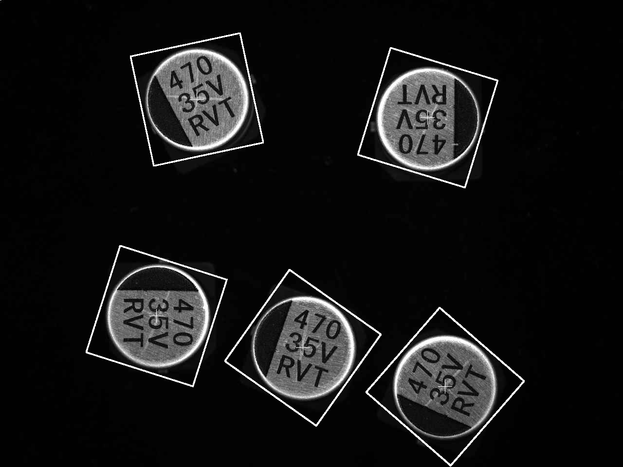
FindGreyImageModel on sample 003: all five capacitors found — crosses mark the subpixel centers, white boxes mark the matched poses — including the nearly \(180^\circ\) flipped instance and the large-angle rotated ones; none is falsely detected on the black background.
The SDK’s measured results on sample 003 are as follows (angles in the SDK’s counterclockwise-positive direction):
| Instance | Position \((x, y)\) | SDK angle | Score |
|---|---|---|---|
| 0 (upright) | \((404.07, 204.06)\) | \(+12.00^\circ\) | 97.58 |
| 1 | \((621.79, 714.39)\) | \(-35.26^\circ\) | 92.87 |
| 2 (flipped) | \((878.39, 241.39)\) | \(+163.00^\circ\) | 91.15 |
| 3 | \((914.14, 794.30)\) | \(+49.00^\circ\) | 90.70 |
| 4 | \((321.08, 649.11)\) | \(-107.66^\circ\) | 89.59 |
All five capacitors score above 89, the angles span the full circle (including a \(+163^\circ\) flipped instance), and the positions are refined to subpixel. Two cross-checks are worth noting. First, the highest peak found by the hand-written fixed \(0^\circ\) template at \(1/2\) resolution (upsampled back to \((404,204)\)) agrees pixel for pixel with the SDK’s instance 0 at \((404.07,204.06)\) — two independent implementations point to the same position. Second, for that same upright instance the fixed-angle NCC is only 0.827, whereas with angle search on the SDK gives 97.58 — angle search recovers the score, exactly the argument of Section 16.3. The same model also finds all five capacitors on samples 004 and 005 (lowest scores 88.9 and 91.2 respectively), confirming the model’s robustness to position and pose changes. The complete runnable project is at code/template_matching/.
Industry Case: Feed Rotation Beyond the Angle Search Range
On an assembly line, a gray-value matching model had its angleExtent set to \(\pm 20^\circ\) at training time according to the incoming material of the day, and it ran stably for months. Then the feeding method changed and the workpieces’ actual rotation reached \(\pm 35^\circ\) — instances beyond the search range had no template pose that could line up at all, match scores plunged below the threshold, and entire batches went undetected. The first reaction was to widen the range straight to the full circle “to be safe”; the result was a marked rise in training time and per-match latency, and worse, with the pose count doubled, similar shapes had more chances to collide with some angle, and the false-detection rate crept up instead. The final solution was to measure the actual rotation distribution of the upstream mechanism, set the range from its envelope plus margin, and add guide rails on the feed track to physically force the rotation back within range. The lesson: the angle search range’s job is to cover physical reality — in this chapter’s samples the capacitors do flip, so the full circle is warranted; but for a pose-constrained station it must not be smaller than the material’s true rotation, and it is emphatically not “the bigger, the safer.”
16.6 Summary
- Template matching = similarity measure + pose search: the measure decides which disturbances it is robust to, and the search dimensions decide which pose variations it can tolerate — neither can be spared.
- SSD/SAD are sensitive to brightness changes (a gain \(g\) brings a residual term of \((g-1)^2\)); NCC subtracts the mean and divides by the standard deviation, and is strictly invariant to linear illumination — measured: dropping one capacitor’s neighbourhood illumination to 50% moves NCC merely from 0.827 to 0.827, while the SSD residual grows 1.5-fold and causes a miss.
- The sharpness of the score-map peak is the localization power; the integer-pixel summit is refined to subpixel by parabola vertex interpolation — in this example the SDK localizes all five capacitors to subpixel with scores above 89.
- NCC has no rotation invariance (under a fixed \(0^\circ\) template the upright instance scores only 0.827 and the flipped instance drops to just over 0.5), so angle must be searched explicitly; here the full circle covers the capacitors’ arbitrary orientation, and with search on the score climbs from 0.827 to 97.58.
- Coarse-to-fine pyramids are the standard means of speeding up matching: a coarse top-level scan plus candidate refinement gave a measured ~100-fold speedup with peak positions exactly identical to the full scan; the ceiling on the level count is that the top-level template must remain recognizable (5 levels automatically here).
NCC’s robustness boundary stops at linear illumination: under nonlinear changes such as specular glare and local shadows, and when the part is partially occluded or changes scale, gray-value matching scores all collapse — those scenarios call for edge-based shape matching, see Chapter 17. How this chapter’s normalized cross-correlation can be computed efficiently with integral images is covered in Lewis’s classic note (Lewis 1995); for template matching within the larger picture of image registration, see Brown’s survey (Brown 1992). For a more systematic treatment of gray-value matching and its acceleration strategies, see further the book by Steger et al. (Steger, Ulrich, and Wiedemann 2018).