Depth-adaptive calibration of line-laser 3D measurement systems using rational polynomial mapping and depth-independent misalignment compensation
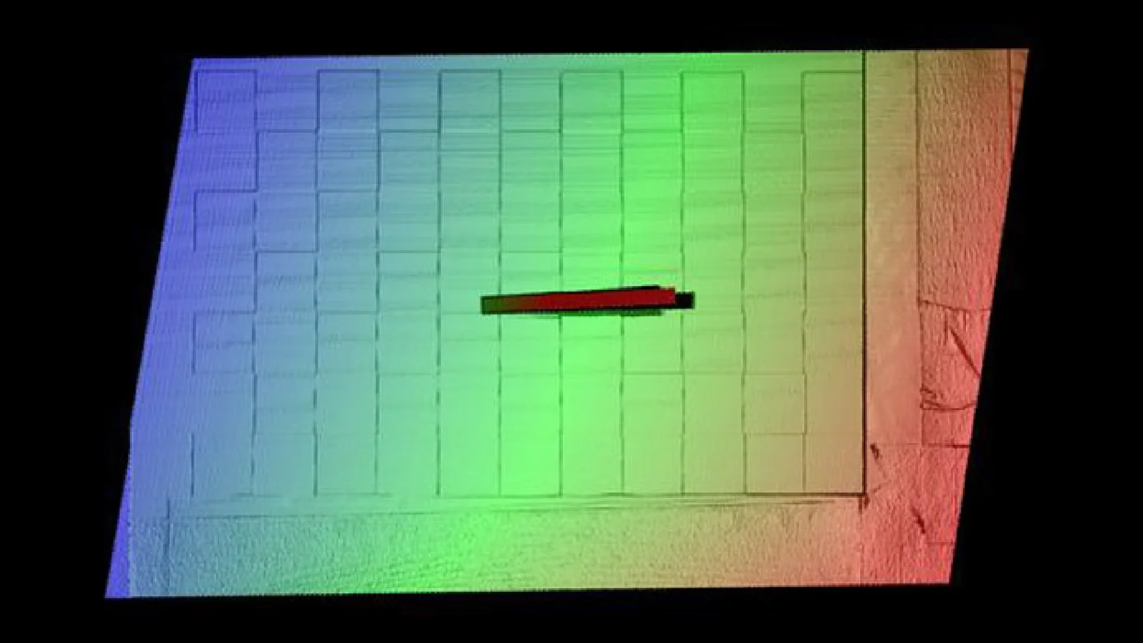
In one sentenceTwo-stage calibration for line-laser 3D sensors: one rational polynomial mapping keeps pixel-to-physical conversion accurate across a 150 mm depth range, and one inverse rotation removes installation shear at every depth.
The problem
A line-laser profiler measures a surface by triangulation. A camera watches the laser stripe on the object and converts each stripe pixel (u, v) into physical coordinates (X, Z) in the laser plane. A full 3D point cloud is then built by stitching many such profiles while a motion stage scans the part. Measurement accuracy is therefore set by calibration, and two different errors erode it across the working depth of field.
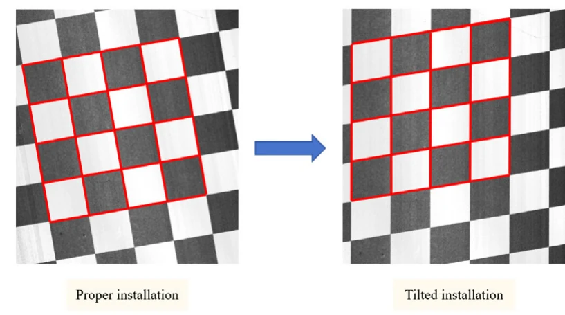
The first error is internal. Conventional calibration rests on a single-plane homography, a strictly linear pixel-to-physical mapping. In a real system, slight tilt of the lifting stage, local non-flatness of the target, radial and tangential lens distortion and stripe-centre extraction noise push the observations away from that ideal perspective, and a pure homography cannot represent the non-linear deviation. The second error is external. If the sensor is not aligned with the motion axis, the stitched cloud carries a systematic shear, and an orthogonal rectangle comes out as a parallelogram. Tuning intrinsics or distortion coefficients cannot remove this shear, and correcting each depth with its own parameters multiplies the parameter count. Existing pipelines usually address either the internal mapping or the external installation geometry, and their joint effect across the depth of field is seldom modelled.
How it works
The method handles the two errors in two separate stages. The internal stage is a one-off factory calibration that fixes the pixel-to-physical mapping inside each profile. The external stage is an on-site compensation that removes the installation shear from the stitched cloud. An automated, motion-triggered workflow runs both, so no manual multi-pose target placement is needed.
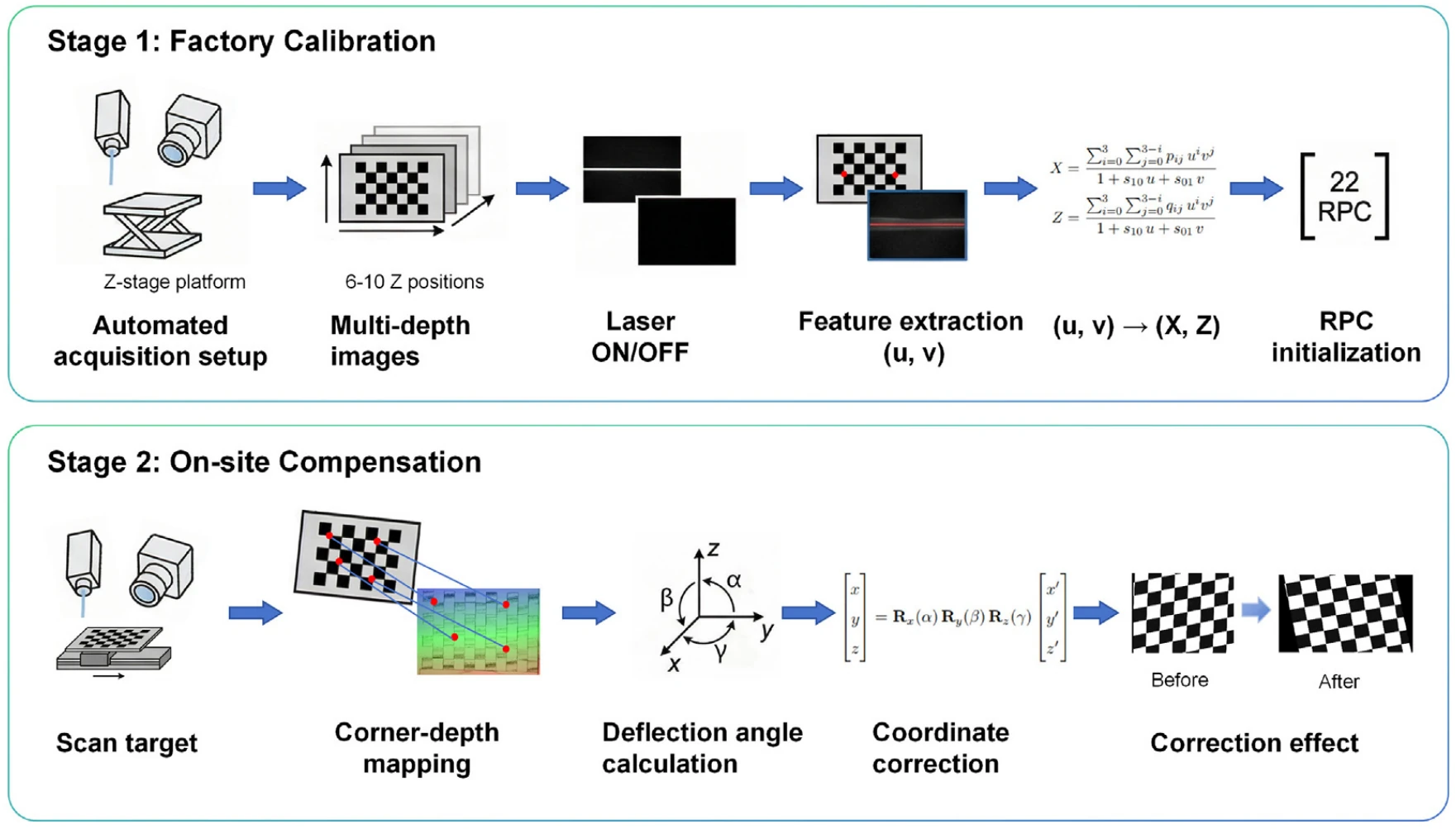
- Sample the full depth range. The camera and line laser are mounted on a precision Z-axis stage that moves through programmed positions. At each height the system captures a laser-on/laser-off image pair, which yields a clean stripe centreline. In the experiments, six depths Z1–Z6 are spaced 30 mm apart over a 150 mm range. Five are used for fitting, and Z3 is held out for testing.
- Fit one rational polynomial mapping. The model keeps the perspective (homography) backbone and adds a bivariate cubic residual in the height direction. Merged into one ratio, it maps (u, v) to X and to Z with a cubic numerator over a shared linear denominator, 22 coefficients in total. Cross-multiplying makes the problem linear, and the correspondences from all training depths form one overdetermined system, solved by least squares.
- Model the shear. The installation error is split into three rotations: roll α, pitch β and yaw γ. With a yaw angle γ, a scan step Δy pushes points sideways by Δx = Δy tan γ, so a rectangle turns into a parallelogram. In the tested push-broom setup, pitch rotates the laser plane about its own axial direction and causes no in-plane shear, so β is set to zero.
- Measure α and γ. A RANSAC line fit to a scan of the empty platform gives a reference line L. Roll comes from a standard height block of nominal height H and width W: α = arctan((H′ − H) / W), where H′ is the measured mean height of its upper face above L. Yaw comes from a checkerboard: requiring adjacent edges of a corrected cell to be perpendicular gives a quadratic equation in sin γ. It is solved for every interior 2 × 2 corner cell, and the median is used.
- Undo the rotation, once for all depths. Every point is mapped through the inverse rotation in Z–Y–X order, Rx(α) Ry(β) Rz(γ), which reduces to Rx(α) Rz(γ) with β = 0. The correction does not depend on depth, so angles estimated once at Z3 are reused across the whole volume.
Results
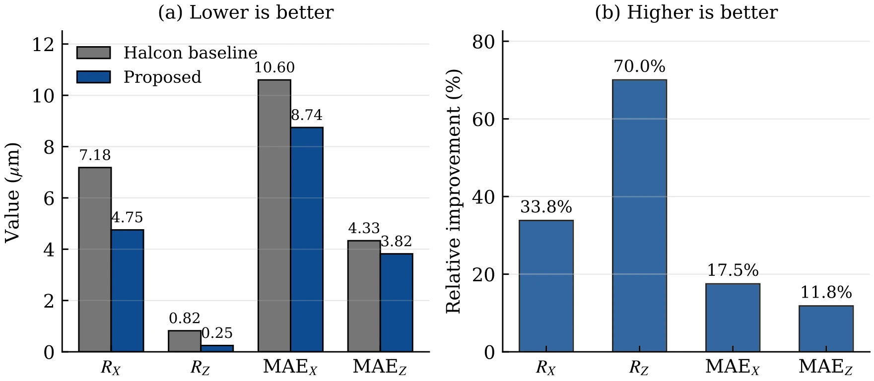
All experiments use one commercial line-laser profiler (OPT-LPF2-006-01) on a programmable Z-stage and a push-broom rig. Ground truth comes from certified standards: a grid distortion target with a 49 × 49 dot array at 1 mm pitch, a metal checkerboard with 25 mm cells, a 25° standard angle block and a height block. For the internal stage, the HALCON baseline and the proposed mapping used the same image stack, the same stripe-centre extractor and the same train/test depth split. Besides the lower mean absolute errors, the proposed mapping improved repeatability by 33.8% in X and 70.0% in Z. The largest gain is in Z repeatability, the metric most sensitive to height-direction nonlinearity, which the cubic residual is designed to absorb.
A sweep over the residual order supports the cubic choice: a quadratic residual underfits, and a quartic one reaches the lowest training error, but its held-out error rises to 12.155 µm in X and 5.130 µm in Z, against 8.745 and 3.820 µm for the cubic residual (Table 11).
For the external stage, the sensor was deliberately tilted (roll α ≈ 5°, yaw γ ≈ 10°) and measured at all six depths in three states: normal installation, tilted without compensation, and tilted with compensation, with 10 trials each. Compared with normal installation, the tilt raised the angle-block error by a factor of 18.84 and the orthogonality error by a factor of 31.87. With the angles frozen from Z3, compensation brought both back to the level of normal installation (0.96× and 0.98× of it). The per-depth reduction stayed within 94.69%–95.04% for the angle and 96.87%–96.97% for orthogonality, so one compensator handles every depth without retuning.
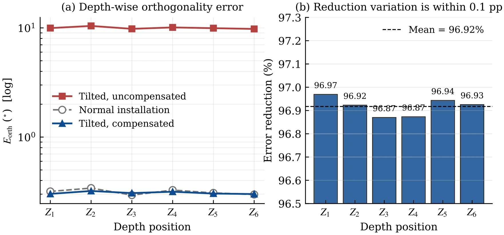
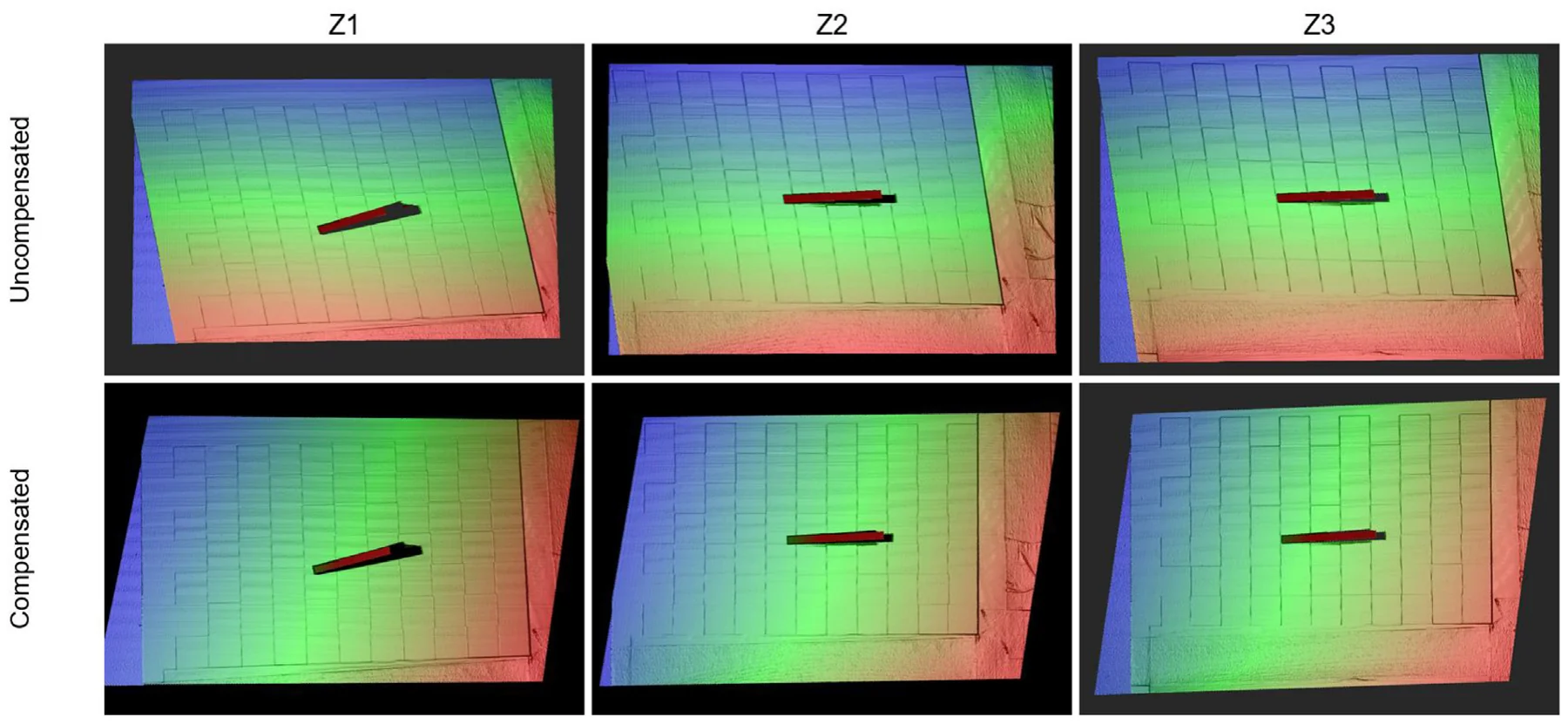
Both stages are needed. With the external compensator disabled, the mapping errors match the full pipeline, but the angle and orthogonality errors stay at their uncompensated levels. With HALCON’s mapping plus the external compensator, the geometric errors drop to 0.0506° and 0.519°, but stay above the full pipeline’s 0.0387° and 0.309°, and the mapping errors return to the baseline (Table 10). The compensator also kept working beyond the vendor’s nominal 5° mounting tolerance: at Z3, with roll swept up to 20° at a yaw of about 10°, the corrected angle error stayed within 0.037°–0.101° and the orthogonality error within 0.16°–0.59° (Table 9). The numerical part of a full calibration takes about 2.3 s, and the total of about 11 minutes is dominated by physical scanning (Table 12).
The authors scope these results to the single tested device and working-distance range. Validation on a second camera, additional standard angles and the repeatability of the estimated angles across independent re-mountings are left to future work.
Cite
@article{cao2026depth,
  title={Depth-adaptive calibration of line-laser 3D measurement systems using rational polynomial mapping and depth-independent misalignment compensation},
  author={Cao, Ling and Lin, Zidong and Yang, Yong and Tang, Quan and Gao, Zhipeng and Feng, Daquan and Pan, Wei},
  journal={Optics \& Laser Technology},
  volume={204},
  pages={116090},
  year={2026},
  doi={10.1016/j.optlastec.2026.116090},
  publisher={Elsevier}
}