Parallel Grayscale Connected Component Analysis via Neighborhood Labeling and Global Region Mapping
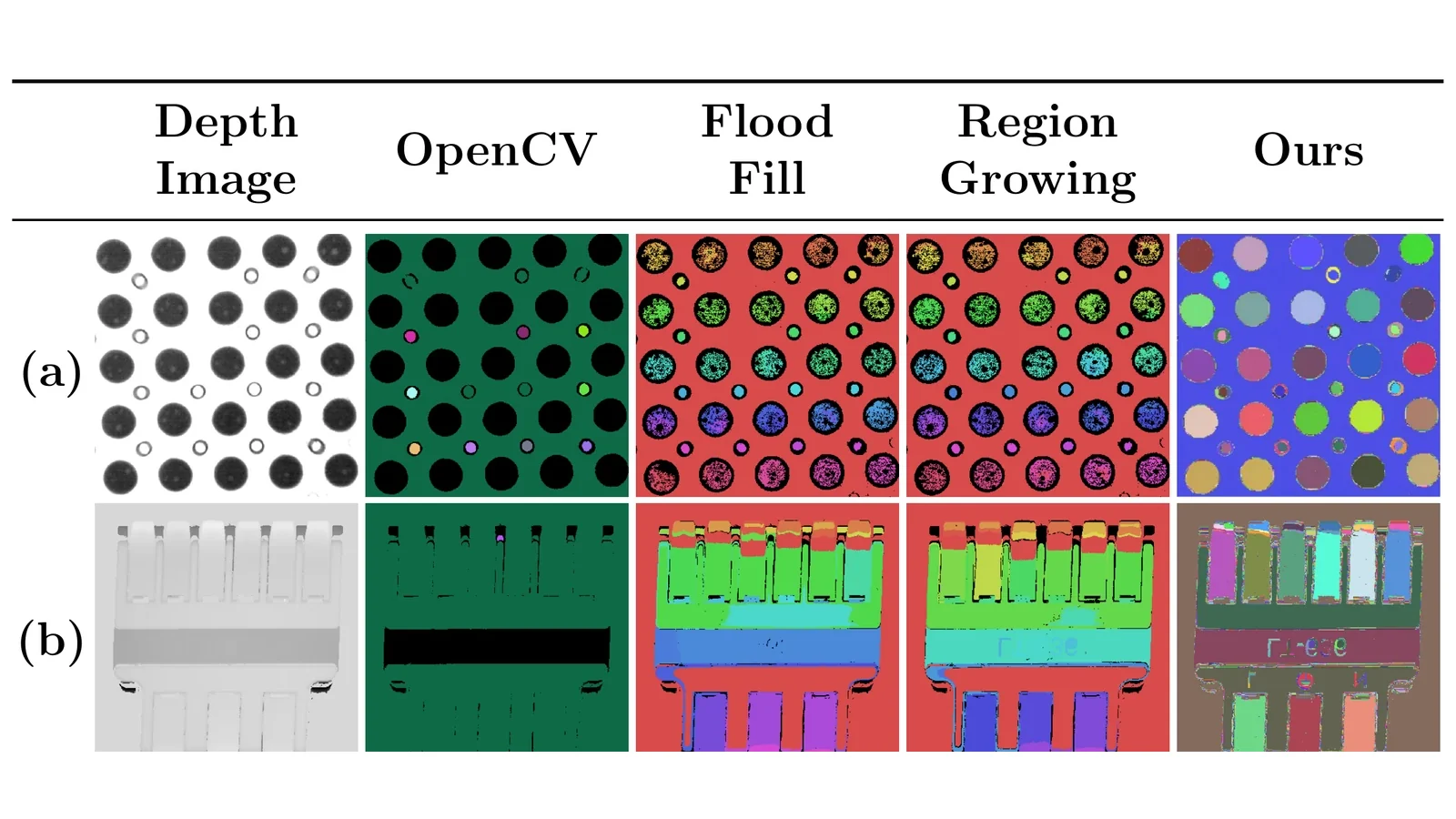
In one sentenceConnected-component labeling on the GPU usually needs a binary image, which throws away grayscale detail. This method labels grayscale and depth images directly, merging regions in a compact region-ID space, and handles a 2-megapixel depth image in about 1.6 ms.
The problem
Connected component analysis (CCA) groups adjacent pixels with similar values into regions. It is a basic step in industrial defect detection, depth-map filtering and medical tissue identification. As sensors reach higher resolutions, industrial lines need it on megapixel images within milliseconds, without losing segmentation fidelity.
The existing options trade one for the other. Serial CPU algorithms such as region growing and flood fill work directly on grayscale intensity and keep fine structure and subtle gradients, but are too slow for high-throughput production lines. Fast GPU algorithms, such as OpenCV’s connectedComponents, are designed for binary images. They need a binarization step first, for example Otsu thresholding, which discards intensity information. Low-contrast defects, or adjacent depth planes with similar intensities, are then merged or lost.
Adapting the binary GPU algorithms to grayscale is not straightforward, according to the authors. Binary images mostly consist of sparse, distinct blobs, whereas grayscale images have dense, continuous gradients. Linking neighbours whose intensities differ by at most a threshold creates far more temporary equivalences between pixels. In label propagation and parallel union-find this leads to heavy atomic contention on global memory, which destroys the parallel speed-up.
How it works
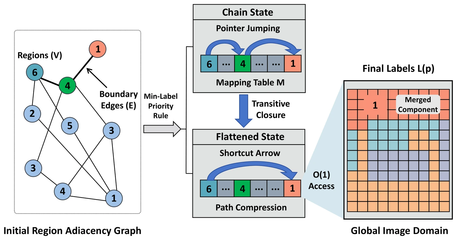
The method runs entirely on the GPU and works on the raw grayscale or depth values. Two neighbouring pixels belong together if their intensities differ by at most a threshold τ. Instead of merging pixel by pixel, it first cuts the image into small local regions, finds where those regions touch, and then merges them in the much smaller space of region IDs.
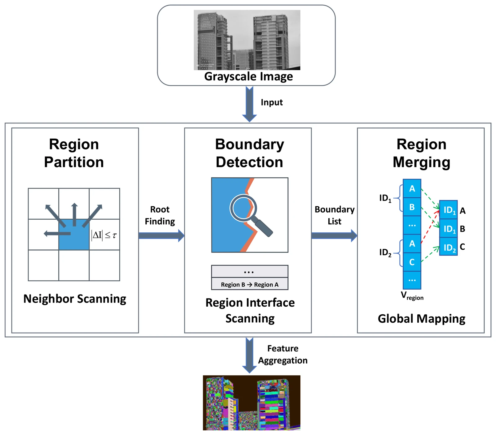
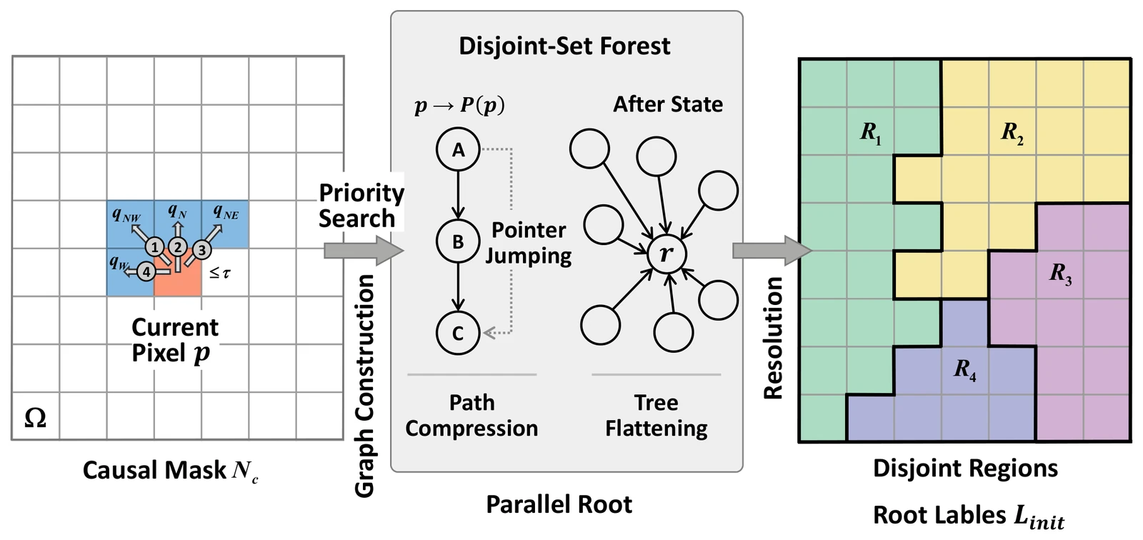
- Local partitioning. Each pixel looks at four neighbours already passed in raster order: upper-left, up, upper-right and left. It attaches to the first one, in that fixed priority order, whose intensity differs by at most τ; if none qualifies, it becomes a root. All pixels decide in parallel. Pointer jumping (path compression) then gives every pixel the ID of its root. Because the mask only looks backwards, some shapes, such as U-shapes, are split into several preliminary regions.
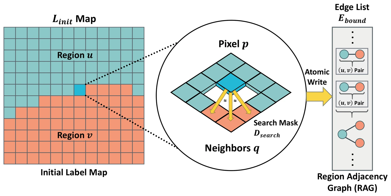
- Boundary detection. To find where those regions should join, each pixel checks its three neighbours below: lower-left, down and lower-right. If a neighbour has a different label but an intensity within τ, the pair of region IDs is written to an edge list with one atomic index increment. The edges form a region adjacency graph, which is much smaller than the image.
- Global region mapping. A mapping table over region IDs starts as the identity. For each edge, the larger ID is mapped to the smaller one; chains are followed to their current roots, so a region connected to several others ends up in one component. A final flattening pass makes every entry point straight to its root, and one pass over the image replaces each pixel’s label by its root.
- Feature aggregation. Region statistics such as the area are counted in each GPU block’s shared memory, in a small hash table, and then added to global memory once per block. This cuts the number of global atomic operations from one per pixel to roughly one per region and block, and the integer sums are exact and deterministic. Components below a minimum area can be filtered out in the same pass.
Results
The algorithm is implemented in CUDA C++ and was tested on an NVIDIA GeForce RTX 3060 with an Intel Core i5-12500 CPU; times are averages of 100 runs and exclude data transfer. The test images are industrial depth maps and grayscale images from 400 × 300 to 4000 × 3000 pixels. The baselines are OpenCV connectedComponents on the GPU, which needs a binary image, and serial region growing and flood fill on the CPU, which work on grayscale like the proposed method.
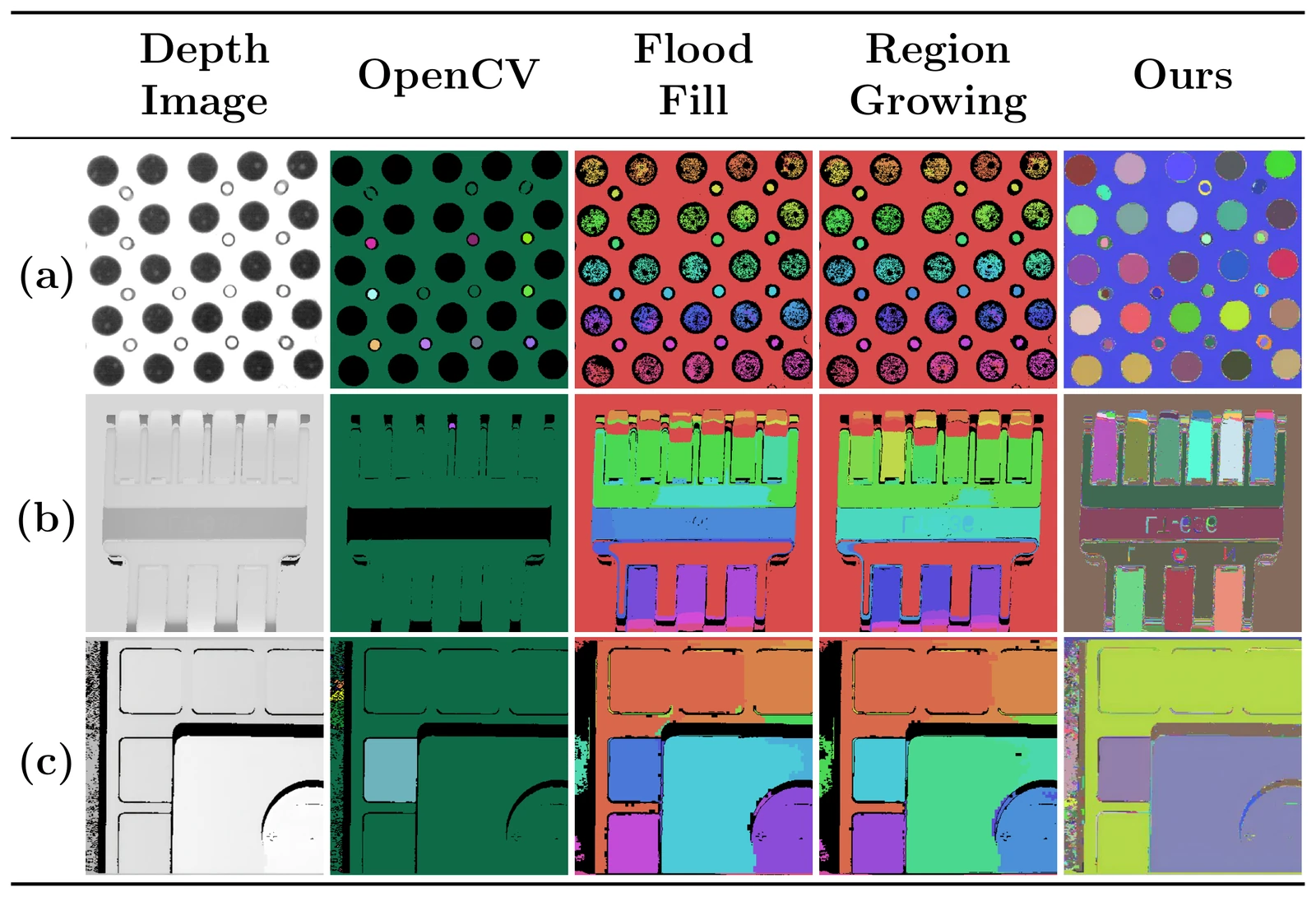
According to the authors, the binary pipeline over-merges or misses subtle grayscale components after thresholding, while the proposed method gives finer region partitions. OpenCV is still much faster, since it labels a binary image: 0.194 ms against 0.865 ms at 1920 × 1080 (Table 2). Against the grayscale baselines the gap is large at every resolution: at 4000 × 3000 the proposed method needs 8.659 ms, region growing 763.75 ms. From 400 × 300 to 4000 × 3000 the pixel count grows 100 times and the runtime 24.4 times, from 0.355 ms to 8.659 ms.
As a correctness check, with binary input and threshold 1 the method finds exactly the same number of components as OpenCV and a classical two-pass algorithm on three test images, with 475, 12,484 and 91,737 components (Table 3). The authors attribute the small differences to region growing in the IoU comparison to floating-point differences between CPU and GPU.
A stage breakdown on a 1920 × 1080 image (Table 5) shows where the time goes: initial labeling 0.608 ms, boundary detection and mapping 0.693 ms, global region-ID merging only 0.028 ms, and final relabeling with statistics 0.165 ms. The threshold τ sets how fine the segmentation is; since the runtime hardly changes with the number of components, it can be tuned without a latency penalty. Because merging is transitive, a gradual intensity ramp stays one component as long as each step between neighbouring pixels is within τ. As future work, the authors name adaptive thresholding, topology-aware boundary rules and multi-GPU extensions.
Cite
@article{cao5854925parallel,
  title={Parallel Grayscale Connected Component Analysis via Neighborhood Labeling and Global Region Mapping},
  author={Cao, Ling and Weng, Jianbo and Lu, Jiawei and Yu, Zihong and Yang, Yong and Feng, Daquan and Pan, Wei},
  journal={Available at SSRN 5854925},
  doi={10.2139/ssrn.5854925}
}